Brass notebook
Created 29 Apr 2013 • Last modified 15 Sep 2013
Initial thinking about data analysis
This shouldn't be a quantitatively intense study, but we are interested in quantifying things rather than finding mere directional effects, so let's think ahead a bit with respect to data analysis.
The DV of chief interest is, for each subject and day, the difference between planned and actual wakeup times. Actual wakeup time will be approximated as report time, the time the subject uses the web form to report that they're awake. Since we're interested in self-control with respect to oversleeping, rather than degrees of grogginess, report time should be discretized to the point that we can distinguish success from failure. Being able to distinguish degrees of failure would be nice but not necessary. Suppose we take each difference and then subtract 10 minutes, to a minimum of 0. Thus successes would be scored as 0s: wakeups no later than 10 minutes after the committed time may be considered close enough. Whereas, reports 10 minutes or more past the committed time likely represent at least a little oversleeping, the standard break provided by a snooze button being 9 minutes. If we use these "snooze times" as-is, then we unfortunately have grogginess-related noise added to the data. Perhaps the report times will end up lumped into clusters separated by intervals of about 10 minutes, which would make it possible to transform them into a number-of-snooze-button-presses score. I guess I'll have to wait and see.
The absolute simplest strategy of data analysis would be to, for each predictor (i.e., score obtained from a pretest), get Spearman correlations between the predictor and the proportion of wakeup committments fulfulled. A next step would be binomial regression on each subject's number of successes. Most sophisticated would be a model in which each wakeup event (put on one of the scales described in the previous paragraph) is modeled individually, including as predictors last night's bedtime and previous wakeup times.
Other commitments should probably be handled with a separate model for each commitment, rather than a multivariate model lumping everything together. A final model can examine dropout as the DV.
Procedure
How much to push the cover story of concern with metabolism can be decided while preparing instructions. Strong emphasis shouldn't be necessary, since it seems unlikely that subjects will anticipate the actual interest in self-control even without much of a cover story.
The Sona study is called "Decision-Making and Habits", and the description says something like "Answer some questionnaires in the lab, then report your daily habits for N weeks." It specifies that subjects will need to go to a website for a few minutes immediately after waking up each day for N weeks, for a total of half a credit in addition to the time in lab. It also says subjects who miss three check-ins will be booted from the study. And it tells subjects to bring any calendar or day planner they might need. In case a subject doesn't read the description, signing up will trigger an email reiterating these special conditions and telling subjects to disenroll otherwise.
In the lab, after signing the consent form, the subject is first asked by the experimenter as to whether they intend to do the check-ins. If they don't say they will, they're asked to leave (and otherwise, they've now made another committment we can track). They're told that they'll get a reminder email tonight, but if they miss two check-ins over the course of the study, they'll be kicked out. (It should be made clear that "missing a check-in" means forgetting to check in, not oversleeping but still checking in promptly after getting up.)
Then the subject gets to the computer. The first question the task program asks is for an email address, since the email address the subject uses for Sona may be out of date. Then the subject makes more commitments. During this process, they should be allowed to use a web browser to access Google Calendar or whatever if they need to. They're asked for things that they intend to spend certain amounts of time on on certain days or every day, such as exercise or studying; let's call these activities "habits". Then the subject fills out a form for each habit and each day in the next N weeks, saying how much time they intend to spend on the habit, rounded to the nearest 15 minutes. For each day, making no commitment is also an option, and there's a box to describe any special circumstances for the day in question. There's a similar form for wakeup times, except with 1-minute instead of 15-minute resolution.
Next, subjects complete the pretests we'll use as predictors. Then they leave.
An email is sent to each subject at 9 pm that evening reminding them of the check-in tomorrow morning. It hints that subjects should load up the check-in webpage on their computer or phone before going to bed. It could also provide a link to a website that can be used to make more reminders.
A check-in is counted as missed if a day goes by with no check-in. An email is sent at the midnight terminating that day, either warning the subject not to forget again or telling the subject they're out of the study.
Although there's no need to provide subjects a way to explicitly drop out other than emailing the experimenters, be sure to think of explicit drop-outs when designing back-end databases and code.
Experimenter instructions
- Assign the subject the next subject number in the Google spreadsheet, recording their first name and birthdate.
- Say "So, as part of this study, you'll need to go to a website and fill out a little form every day after you wake up for the next two weeks. Do you agree to do that?"
- If the subject doesn't agree, send them away.
- Have the subject fill out the consent form.
- Lead the subject to a testing computer.
- Drag "exp.py" (in the folder "Brass" in "tasks") onto the DrPython icon. Launch the program, then minimize the DrPython window.
- Point out to the subject the Firefox icon on the desktop, in case they need a web browser.
- Once the subject is done:
- Don't provide any debriefing (the study isn't over yet).
- Tell the subject they'll get an email at 9 pm tonight that will tell them how to check in.
- On the testing computer, quit Firefox if it's open, and un-minimize the DrPython window so you're ready for the next subject.
Pretests
- Economics preferences test - maybe just use the Hazel battery
- Patience
- Stationarity
- Risk aversion
- Loss aversion
- Consideration of Future Consequences Scale (Strathman, Gleicher, Boninger, & Edwards, 1994)
- Contentiousness (John, Naumann, & Soto, 2008)
- Impulse control / executive function? (Stroop; MSIT)
Scoring pretest performance
In each of the econometric tests, choices could be perhaps most simply modeled as
where m and b are parameters and x is some transformation of the ratio of amounts; say, the log thereof. The x-value for which a subject is indifferent is then the most obvious basis for scoring this test. We'd define each subject's patience, risk aversion, or whatever as an estimate of this value. Setting and solving for x, we get x = −b/m.
A logical way to parametrize this choice model would be in terms of the indifference point (analogous to the mean) and some measure of how fast the choice probability changes as the input changes (analogous to the variance). Call the former μ. For the latter, let's use the difference in x-values that makes a 1-logit difference and call it ι. Solving , solving for x, and subtracting μ, we get ι = 1 / a. We can now say:
If we parametrize with ρ = 1 / ι instead, we get:
In practice, it looks like we could get each subject's score by estimating (ρ, μ) and discarding ρ. Or we could use the standard parametrization and calculate μ = −b/m. Whichever's easier using the parameter-estimation technique in question.
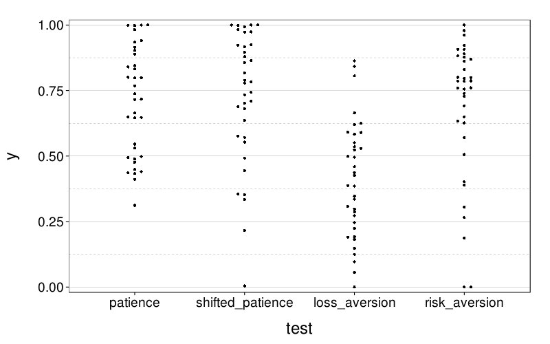
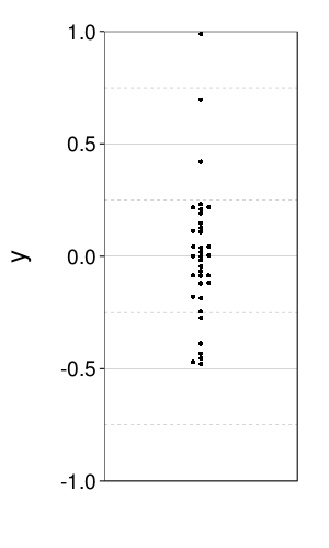
Descriptive econometric scores
eips = econ.indiff.per.s(econg)
dodge(test, y, data = ss(eips, test != "stationarity")) +
    coord_cartesian(ylim = c(-.02, 1.02))
dodge(1, y, data = ss(eips, test == "stationarity")) +
    coord_cartesian(xlim = c(.75, 1.25), ylim = c(-1, 1))
Wakeup outcomes
There's a variety of different overall outcomes possible for each subject:
- Explicitly leaving the study (but this has never happened yet and may well never happen)
- Getting kicked out (after missing two check-ins)
- Missing one check-in
- Missing no check-ins
Among subjects who leave the study, voluntarily or by being kicked out, we can ask how many days they lasted.
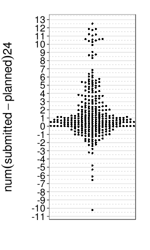
For each day the subject planned a wakeup time and checked in, we can ask what the difference is between their planned time and check-in time. Here's a plot of these differences, in hours:
dodge(1, num(submitted - planned) * 24, data =
        ss(wakeups, !is.na(planned) & !is.na(submitted))) +
    scale_y_continuous(breaks = seq(-20, 20, 1)) +
    coord_cartesian(xlim = 1 + c(-.25, .25))
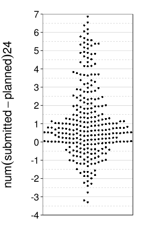
Zooming in:
dodge(0, num(submitted - planned) * 24, data =
        ss(wakeups, !is.na(planned) & !is.na(submitted))) +
    scale_y_continuous(breaks = seq(-4, 7, 1)) +
    coord_cartesian(ylim = c(-4, 7), xlim = 1 + c(-.25, .25))
Define a subject's wakeup score as follows. First, define a P-day as a day for which the subject in question (1) planned a wakeup time and (2) didn't drop out before reaching that day. Let n be the subject's number of P-days. Let s be the number of successes; a P-day is counted as a success iff the subject checked in and the checkin time was no more than half an hour past the planned wakeup time. Then the subject's wakeup score, w, is (s + 1) / (n + 2). (This number is the posterior mean of a Bernoulli-distributed random variable with a flat prior and s observed successes in n trials.)
Unfortunately, w doesn't really suffice as a measure of observed self-control for wakeup times, because of kickouts. Kickouts lower n and therefore bring w closer to 1/2 although I want to treat a kickout as evidence of lower, not more moderate, self-control. So let's try to predict not w but the pairs (w, d), where d is 1 if the subject was kicked out and 0 otherwise.
Predicting wakeup scores and kickouts
wud = as.data.frame(as.matrix(ss(   # Numify every column
    cbind(ss(sb, good)[qw(wus, plannedwu, cfc, con)],
        dcast(econ.indiff.per.s(econg), s ~ test, value.var = "y")[,-1]),
    !is.na(wus))))

kod = cbind(
    data.frame(ko = !is.na(ss(sb, good)$kicked)),
    as.data.frame(as.matrix(ss(   # Numify every column
        cbind(ss(sb, good)[qw(wus, plannedwu, cfc, con)],
            dcast(econ.indiff.per.s(econg), s ~ test, value.var = "y")[,-1])))))
The sample sizes are:
data.frame(row.names = qw(wud, kod), sample.size = c(nrow(wud), nrow(kod)))
| sample.size | |
|---|---|
| wud | 27 |
| kod | 34 |
The base rates for kickouts are:
table(kod$ko)
| count | |
|---|---|
| FALSE | 26 |
| TRUE | 8 |
Wakeup scores only
Simple linear model
We begin with a linear model predicting w from the number of days with planned wakeup times, the four econometric scores, and the two personality tests.
fit = lm(data = wud, logit(wus) ~
    plannedwu + cfc + con +
    patience + stationarity + loss_aversion + risk_aversion)
round(summary(fit)$r.squared, 2)
| value | |
|---|---|
| 0.4 |
That's not terrible, but not enough for precise prediction. Notice that:
round(ilogit(quantile(logit(wud$wus), c(.025, .975))), 2)
| value | |
|---|---|
| 2.5% | 0.15 |
| 97.5% | 0.85 |
and
round(ilogit(predict(fit, interval = "prediction")), 2)
| fit | lwr | upr | |
|---|---|---|---|
| s002 | 0.35 | 0.07 | 0.81 |
| s003 | 0.34 | 0.06 | 0.81 |
| s004 | 0.43 | 0.09 | 0.85 |
| s005 | 0.38 | 0.08 | 0.82 |
| s007 | 0.22 | 0.03 | 0.73 |
| s008 | 0.34 | 0.06 | 0.81 |
| s009 | 0.38 | 0.07 | 0.83 |
| s011 | 0.45 | 0.08 | 0.89 |
| s012 | 0.28 | 0.03 | 0.81 |
| s013 | 0.43 | 0.08 | 0.87 |
| s014 | 0.65 | 0.16 | 0.95 |
| s015 | 0.20 | 0.02 | 0.73 |
| s016 | 0.51 | 0.10 | 0.90 |
| s017 | 0.49 | 0.10 | 0.89 |
| s018 | 0.59 | 0.16 | 0.92 |
| s019 | 0.42 | 0.09 | 0.85 |
| s020 | 0.36 | 0.07 | 0.81 |
| s021 | 0.32 | 0.06 | 0.78 |
| s023 | 0.60 | 0.15 | 0.93 |
| s024 | 0.43 | 0.09 | 0.85 |
| s025 | 0.56 | 0.12 | 0.92 |
| s026 | 0.43 | 0.09 | 0.85 |
| s027 | 0.83 | 0.32 | 0.98 |
| s028 | 0.52 | 0.12 | 0.90 |
| s029 | 0.25 | 0.03 | 0.76 |
| s030 | 0.31 | 0.05 | 0.79 |
| s031 | 0.51 | 0.11 | 0.90 |
so the uncertainty in new wakeup scores, given predictors equal in value to what we have here, is no smaller than the overall variability in wakeup scores.
With two-way interactions
fit = lm(data = wud, logit(wus) ~
    (plannedwu + cfc + con +
    patience + stationarity + loss_aversion + risk_aversion)^2)
round(summary(fit)$r.squared, 2)
| value | |
|---|---|
| 1 |
Whoops, we already have more terms (1 + 7 choose 1 + 7 choose 2 = 29) than data points.
Ridge regression
set.seed(1)
lambda2 = optL2(data = wud,
    logit(wus) ~ (plannedwu + cfc + con +
        patience + stationarity + loss_aversion + risk_aversion)^2,
    model = "linear", standardize = T, fold = 5)$lambda
fit = penalized(data = wud,
    logit(wus) ~ (plannedwu + cfc + con +
        patience + stationarity + loss_aversion + risk_aversion)^2,
    model = "linear", standardize = T, lambda2 = lambda2)
round(coef(fit)[order(-abs(coef(fit)))], 3)[1:5]

# y = logit(wud$wus)
# round(digits = 2,
#     1 - sum(residuals(fit)^2) / sum((y - mean(y))^2))
#   # R-squared
| value | |
|---|---|
| (Intercept) | -0.205 |
| risk_aversion | -0.024 |
| patience:risk_aversion | -0.020 |
| patience:loss_aversion | 0.008 |
| loss_aversion:risk_aversion | -0.004 |
These are the five biggest coefficients. That is a pretty conservative model.
MARS
efit = earth(logit(wus) ~ plannedwu + cfc + con + patience + stationarity + loss_aversion + risk_aversion, data = wud, degree = 2, trace = 1, nprune = 5, penalty = -1, pmethod = "exhaustive")
Fake prediction intervals by adding `quantile(resid(earthfit), c(.025, .975))` to predicted means.
Kickout only
Logistic regression
fit = glm(data = kod, ko ~
    plannedwu + cfc + con +
    patience + stationarity + loss_aversion + risk_aversion)
round(sort(ilogit(predict(fit))), 2)
| value | |
|---|---|
| s004 | 0.43 |
| s015 | 0.47 |
| s018 | 0.48 |
| s005 | 0.50 |
| s014 | 0.51 |
| s001 | 0.53 |
| s003 | 0.57 |
| s007 | 0.58 |
| s017 | 0.59 |
| s008 | 0.59 |
| s002 | 0.61 |
| s019 | 0.63 |
| s009 | 0.65 |
| s021 | 0.66 |
| s013 | 0.69 |
| s016 | 0.70 |
| s020 | 0.73 |
| s012 | 0.74 |
| s011 | 0.75 |
These probabilities are far from 0 and 1, so the predictions are weak.
Logistic ridge regression (with interactions)
set.seed(1)
lambda2 = optL2(data = kod,
    ko ~ (plannedwu + cfc + con +
        patience + stationarity + loss_aversion + risk_aversion)^2,
    model = "logistic", standardize = T, fold = 5)$lambda
fit = penalized(data = kod,
    ko ~ (plannedwu + cfc + con +
        patience + stationarity + loss_aversion + risk_aversion)^2,
    model = "logistic", standardize = T, lambda2 = lambda2)
round(sort(predict(fit, data = kod)), 2)
| value | |
|---|---|
| s015 | 0.22 |
| s004 | 0.24 |
| s005 | 0.24 |
| s018 | 0.27 |
| s001 | 0.28 |
| s014 | 0.32 |
| s007 | 0.35 |
| s017 | 0.39 |
| s002 | 0.39 |
| s016 | 0.40 |
| s003 | 0.44 |
| s008 | 0.44 |
| s009 | 0.45 |
| s019 | 0.46 |
| s021 | 0.51 |
| s013 | 0.58 |
| s011 | 0.61 |
| s012 | 0.70 |
| s020 | 0.72 |
A little better, I'd say, but not much.
Activity coding
I've coded each activity as a "virtue" (e.g., "Exercise"), a "vice" (e.g., "Video Games"), or unknown (e.g., "Reading"). This distinction is important for how to interpret people's commitments. In the case of a virtue activity, clearly, a person fulfills their commitment when they spend the amount of time they planned to spend or more on the activity. In the case of a vice activity, conversely, I figure a person fulfills their commitment when they spend the amount of time they planned to spend or less on the activity. Thus, I construe exercising more than planned as a self-control success and playing video games more than planned as a self-control failure. This construal is what the coding represents; when I code an activity as unknown, that means I don't know which way to construe any gaps between plans and actions for that activity.
In the activity-listing instructions, I wrote "Don't include activities you're obliged to do and don't especially want to accomplish. For example, you might spend an hour every day commuting, but you probably aren't interested in commuting for its own sake." People included things like "Work" anyway. Does it take self-control to go to work? It's hard to say; it depends on the person (and the job). So, I haven't attempted to treat these activities specially.
Christian brought up one problem with including both virtues and vices in analyses, which is handling the trade-off between them. Imagine Joe commits to 2 hours of studying (a virtue) and 2 hours of watching TV (a vice). If he ended up doing (a) 15 minutes of studying and 15 minutes of TV-watching or (b) 15 min of studying and 1 hour 15 minutes of TV-watching, he'd be failing the virtue commitment and fulfilling the vice commitment either way. But (b) suggests less self-control because it gives a stronger impression than (a) that Joe spent time on a vice that he could've spent on a virtue. My way around this issue, for now, is to simply exclude vices from analysis.
I figure I shouldn't give a grace period for activities the way I give a half-hour grace period for wakeup times, since I told subjects to round answers to the nearest 15 minutes.
One-dimensional self-control scores
Multivariate data analysis is hard, particularly with unlike datatypes. Here's another approach. For each subject, we'll assign a single "self-control score" (SCS) which represents, intuitively, the proportion of commitments the subject fulfills. Define (using, again, the formula for the posterior mean of a Bernoulli distribution) scs = (s + 1) / (n + 2), where n is the number of commitments and s the number of successes (i.e., the number of commitments fulfilled). (Alternatively, instead of doing regression on SCS itself, we can do real binomial regression with n and s.) n is incremented by 1 for each:
- day the subject is supposed to check in
- scheduled wakeup time
- scheduled span of time spent on a virtuous activity
Category 1 always contributes 14 units to n, since the study lasts 2 weeks. Items in category 2 and category 3 are not counted if the subject didn't check in on the day in question, since we have no data. It's still better to check in late than not check in at all, though: if you check in late, n is incremented by 2 (one for category 1 and one for category 2) and s is incremented by 1 (for checking in), so your SCS shifts towards 1/2, whereas if you don't check in, n is incremented by 1 and s is unchanged, so your SCS shifts towards 0.
I'm ignoring kickouts, such that kicked-out subjects are treated as having missed all subsequent checkins. Of course, this data-analysis strategy suggests against kicking people out. Perhaps I'll change that in the next round of data collection.
Predicting SCS
(Or not, if we're going with sc.p instead.)
scd = as.data.frame(as.matrix(   # Numify every column
    supplement(
        ss(sb, good)[qw(sc.p, sc.n, sc.s, cfc, con)],
        dcast(econ.indiff.per.s(econg), s ~ test, value.var = "y"))))
Baseline
Suppose I tried to predict sc.p with a single interval for all subjects. How wide would it have to be? (This is only a lower bound, since I'm only looking at training error.)
qs = unname(quantile(scd$sc.p, c(.025, .975)))
round(d = 3, c(
    lo = qs[1],
    hi = qs[2],
    diff = qs[2] - qs[1],
    coverage = mean(scd$sc.p >= qs[1] & scd$sc.p <= qs[2])))
| value | |
|---|---|
| lo | 0.272 |
| hi | 0.872 |
| diff | 0.599 |
| coverage | 0.944 |
That's very wide. Let's try a somewhat less stupid baseline in which we posit a single probability of fulfilling commitments, and then we construct per-subject intervals from the binomial distribution.
with(scd,
   {ml = optimize(
        function(p) -sum(dbinom(sc.s, sc.n, p, log = T)),
        c(.001, .999))$minimum
    nc = optimize(interval = c(.99, .995), function(nc)
      {lo = qbinom((1 - nc)/2, sc.n, ml)/sc.n
       hi = qbinom(1 - (1 - nc)/2, sc.n, ml)/sc.n
       abs(.95 - mean(lo <= sc.p & sc.p <= hi)) +
           .1 * median(hi - lo)})$minimum
    assess.prop.intervals(sc.s/sc.n,
        qbinom((1 - nc)/2, sc.n, ml)/sc.n,
        qbinom(1 - (1 - nc)/2, sc.n, ml)/sc.n)})
| x | |
|---|---|
| Widths Q1 | 0.37 |
| Widths Q3 | 0.5 |
| Coverage | 92% (33 of 36) |
Still pretty wide.
Logistic regression
We use sc.p instead of proper binomial regression (with sc.s and sc.n) so all subjects are treated equally.
fit = glm(data = scd, family = quasibinomial(link = "logit"),
    sc.p ~
        cfc + con +
        patience + stationarity + loss_aversion + risk_aversion)
d = binom.intervals(scd$sc.n, predict(fit, type = "response"))
assess.prop.intervals(scd$sc.s/scd$sc.n, d[,"lo"], d[,"hi"])
# d = binom.intervals = function(n, ps)
#     cbind(
#         lo = qbinom(.025, n, ps)/n,
#         hi = qbinom(.975, n, ps)/n)
# with(ss(sb, good), plot.sc.preds(sc.n, sc.s,
#     predict(fit, type = "response")[row.names(ss(sb, good))]))
| x | |
|---|---|
| Widths Q1 | 0.28 |
| Widths Q3 | 0.38 |
| Coverage | 78% (28 of 36) |
Coverage is insufficient, probably because the intervals don't account for sampling error. Let's try bootstrapping.
d = replicate(1e4, with(samprows(scd, rep = T),
   {fit = glm(data = scd, family = quasibinomial(link = "logit"),
        sc.p ~
            cfc + con +
            patience + stationarity + loss_aversion + risk_aversion)
    rbinom(nrow(scd), scd$sc.n, predict(fit, type = "response"))/scd$sc.n}))
d = t(apply(d, 1, function(v) quantile(v, c(.025, .975))))
assess.prop.intervals(scd$sc.s/scd$sc.n, d[,1], d[,2])
| x | |
|---|---|
| Widths Q1 | 0.28 |
| Widths Q3 | 0.38 |
| Coverage | 78% (28 of 36) |
Well, that didn't work, and I'm not entirely sure why.
Gotta go Bayes. But arm and MCMCpack don't allow sampling from the posterior predictive distribution. I think I should write a wrapper function or two for Stan.
Nah, since Stan doesn't have very good facilities for prediction, either. Let's implement a way to do prediction with arm or so.
fit = glm(data = scd, family = binomial(link = "logit"),
    cbind(sc.s, sc.n - sc.s) ~
        cfc + con +
        patience + stationarity + loss_aversion + risk_aversion)
post = sim.y.mu(fit, model.frame(fit), 1e4)
d = sapply(row.names(scd), function(s)
    quantile(rbinom(ncol(post), scd[s, "sc.n"], post[s,])/scd[s, "sc.n"],
        c(.025, .975)))
assess.prop.intervals(scd$sc.s/scd$sc.n, d[1,], d[2,])
| x | |
|---|---|
| Widths Q1 | 0.31 |
| Widths Q3 | 0.4 |
| Coverage | 81% (29 of 36) |
Well, that's something, at least. Let's estimate the predictive accuracy of this model with cross-validation.
d = cv.intervals(scd, K = 10, f = function(d.train, d.test)
   {fit = glm(data = d.train, family = binomial(link = "logit"),
        cbind(sc.s, sc.n - sc.s) ~
            cfc + con +
            patience + stationarity + loss_aversion + risk_aversion)
    post = sim.y.mu(fit, d.test, 1e4)
    t(sapply(row.names(d.test), function(s)
        quantile(rbinom(ncol(post), d.test[s, "sc.n"], post[s,])/d.test[s, "sc.n"],
        c(.025, .975))))})
assess.prop.intervals(scd$sc.p, d[,1], d[,2])
| x | |
|---|---|
| Widths Q1 | 0.32 |
| Widths Q3 | 0.42 |
| Coverage | 69% (25 of 36) |
With all two-way interactions, linear
fit = lm(data = scd, sc.p ~
     (cfc + con +
      patience + stationarity + loss_aversion + risk_aversion)^2)
post = sim.y.mu(fit, model.frame(fit), 2e4)
d = sapply(row.names(scd), function(s) quantile(post[s,], c(.025, .975)))
assess.prop.intervals(scd$sc.p, d[1,], d[2,])
| x | |
|---|---|
| Widths Q1 | 0.32 |
| Widths Q3 | 0.47 |
| Coverage | 89% (32 of 36) |
With all two-way interactions, logistic
fit = glm(data = scd, family = binomial(link = "logit"),
        cbind(sc.s, sc.n - sc.s) ~
            (cfc + con +
            patience + stationarity + loss_aversion + risk_aversion)^2)
post = sim.y.mu(fit, model.frame(fit), 2e4)
d = sapply(row.names(scd), function(s)
    quantile(rbinom(ncol(post), scd[s, "sc.n"], post[s,])/scd[s, "sc.n"],
       c(.025, .975)))
assess.prop.intervals(scd$sc.p, d[1,], d[2,])
| x | |
|---|---|
| Widths Q1 | 0.34 |
| Widths Q3 | 0.44 |
| Coverage | 97% (35 of 36) |
Coverage is good, but the intervals aren't much narrower than for baseline.
Again, using cross-validation to estimate predictive accuracy:
d = cv.intervals(scd, K = 10, f = function(d.train, d.test)
   {fit = glm(data = d.train, family = binomial(link = "logit"),
        cbind(sc.s, sc.n - sc.s) ~
            (cfc + con +
            patience + stationarity + loss_aversion + risk_aversion)^2)
    post = sim.y.mu(fit, d.test, 1e4)
    t(sapply(row.names(d.test), function(s)
        quantile(rbinom(ncol(post), d.test[s, "sc.n"], post[s,])/d.test[s, "sc.n"],
        c(.025, .975))))})
assess.prop.intervals(scd$sc.p, d[,1], d[,2])
| x | |
|---|---|
| Widths Q1 | 0.4 |
| Widths Q3 | 0.62 |
| Coverage | 75% (27 of 36) |
The big drop in coverage is no big surprise; I expected a model with this many predictors to overfit. At the same time, the intervals are really wide. I daresay this is not a good model.
With all two-way interactions, logistic ridge
ridgebayes.2waylog = function(data)
    bayesglm.cv.ps(scd, "sc.p", K = 10,
         cbind(sc.s, sc.n - sc.s) ~
             (cfc + con +
             patience + stationarity + loss_aversion + risk_aversion)^2,
         family = binomial(link = "logit"),
         prior.df = Inf,
         prior.scale.for.intercept = Inf, prior.df.for.intercept = Inf)
l = cached(ridgebayes.2waylog(scd))
post = sim.y.mu(l$fit, model.frame(l$fit), 2e4)
d = sapply(row.names(scd), function(s)
    quantile(rbinom(ncol(post), scd[s, "sc.n"], post[s,])/scd[s, "sc.n"],
       c(.025, .975)))
assess.prop.intervals(scd$sc.p, d[1,], d[2,])
| x | |
|---|---|
| Widths Q1 | 0.31 |
| Widths Q2 | 0.39 |
| Coverage | 81% (29 of 36) |
Now for predictive validity. This involves optimization via cross-validation inside each outer cross-validation fold, so it's really slow.
i = 0
d = cached(cv.intervals(scd, K = 10, f = function(d.train, d.test)
   {i <<- i + 1
    message("fold ", i)
    l = ridgebayes.2waylog(d.train)
    post = sim.y.mu(l$fit, d.test, 1e4)
    t(sapply(row.names(d.test), function(s)
        quantile(rbinom(ncol(post), d.test[s, "sc.n"], post[s,])/d.test[s, "sc.n"],
        c(.025, .975))))}))
assess.prop.intervals(scd$sc.p, d[,1], d[,2])
| x | |
|---|---|
| Widths Q1 | 0.3 |
| Widths Q2 | 0.4 |
| Coverage | 75% (27 of 36) |
An improvement over the unpenalized model: coverage is similar, but intervals are narrower.
plot.sc.preds(scd$sc.p, d[,1], d[,2])
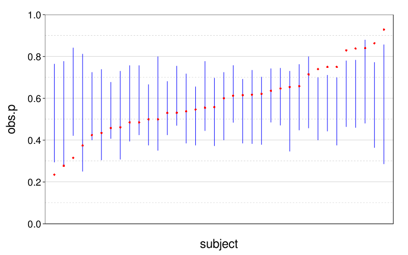
The figure suggests we are not meaningfully predicting individual differences.
References
John, O. P., Naumann, L. P., & Soto, C. J. (2008). Paradigm shift to the integrative Big Five trait taxonomy: History, measurement, and conceptual issues. In O. P. John, R. W. Robins, & L. A. Pervin (Eds.), Handbook of personality: Theory and research (3rd ed., pp. 114–158). New York, NY: Guilford Press. ISBN 978-1-59385-836-0. Retrieved from http://www.ocf.berkeley.edu/~johnlab/2008chapter.pdf
Strathman, A., Gleicher, F., Boninger, D. S., & Edwards, C. S. (1994). The consideration of future consequences: Weighing immediate and distant outcomes of behavior. Journal of Personality and Social Psychology, 66(4), 742–752. doi:10.1037/0022-3514.66.4.742