The predictive accuracy of intertemporal-choice models
Kodi B. Arfer and Christian C. Luhmann
Created 4 Mar 2013 • Last modified 26 Feb 2015
How do people choose between a smaller reward available sooner and a larger reward available later? Past research has evaluated models of intertemporal choice by measuring goodness of fit or identifying which decision-making anomalies they can accommodate. An alternative criterion for model quality, which is partly antithetical to these standard criteria, is predictive accuracy. We used cross-validation to examine how well 10 models of intertemporal choice could predict behavior in a 100-trial binary-decision task. Many models achieved the apparent ceiling of 85% accuracy, even with smaller training sets. When noise was added to the training set, however, a simple logistic-regression model we call the difference model performed particularly well. In many situations, between-model differences in predictive accuracy may be small, contrary to longstanding controversy over the modeling question in research on intertemporal choice, but the simplicity and robustness of the difference model recommend it to future use.
Acknowledgments: We wish to thank Luis E. Ortiz for his guidance on data analysis.
This paper was published as:
Arfer, K. B., & Luhmann, C. C. (2015). The predictive accuracy of intertemporal-choice models. British Journal of Mathematical and Statistical Psychology, 68, 326–341. doi:10.1111/bmsp.12049
The official PDF has only minor differences from this the original document, such as the use of British spelling.
Introduction
People frequently need to choose between one outcome available soon (the smaller sooner, or SS, option) and a more desirable outcome available later (the larger later, or LL, option). Deciding whether to indulge in a dessert or stick to a diet, to splurge on an impulse buy or save up for a more desirable item, and to relax or study for an upcoming exam, can all be characterized as intertemporal choices. Accordingly, laboratory measures of individual differences in intertemporal preferences have been associated with variables such as body-mass index (Sutter, Kochaer, Rützler, & Trautmann, 2010), credit-card debt (Meier & Sprenger, 2010), heroin addiction (Madden, Petry, Badger, & Bickel, 1997), and diagnoses of attention-deficit disorder (Demurie, Roeyers, Baeyens, & Sonuga‐Barke, 2012).
Extant models of intertemporal choice
Despite the real-world relevance of laboratory measures of intertemporal choice, the question of how to quantitatively model such choices, even in simple laboratory tasks, is far from settled (see Doyle, 2013, for a broad survey, but see also Bleichrodt, Potter van Loon, Rohde, & Wakker, 2013). Samuelson (1937) influentially proposed that people discount rewards based on the delay until their receipt. According to this proposal, $100 to be received a month in the future is treated as equivalent to some smaller amount of money available now, its immediacy equivalent. A discounting function f maps delays to numbers in [0, 1] called discount factors, which ultimately determine the immediacy equivalent of any delayed reward. For example, f(1 month) • $100 would yield the immediacy equivalent of $100 delayed by 1 month. In a binary forced-choice task, it is assumed that people will prefer the option with the greater discounted value.
The most thoroughly studied discounting function, from both descriptive and normative perspectives, is the exponential function. An exponential discounting function is of the form where the discount rate, k ∈ [0, ∞), is a free parameter typically assumed to vary across subjects. Among the normatively appealing features of exponential discounting is dynamic consistency: given a pair of delayed rewards, an exponential discounter's preference will never reverse merely from the passage of time (Koopmans, 1960). However, humans have been found to be dynamically inconsistent: someone who prefers $110 in a year and a month over $100 in a year may also prefer $100 today over $110 in a month, suggesting a reversal of preferences over the course of a year (e.g., Green, Fristoe, & Myerson, 1994; Kirby & Herrnstein, 1995). The importance of dynamic inconsistency is suggested by its real-world consequences. On New Year's Eve, one might prefer starting an exercise routine to slacking off on the following Monday, but then, when Monday arrives, one's mind may change. Indeed, dynamic inconsistency has been identified as the econometric manifestation of failures of self-control (Rachlin, 1995; Luhmann & Trimber, 2014).
An alternative discounting function is a hyperbolic function of the form where the discount rate, k ∈ [0, ∞), is a free parameter (Chung & Herrnstein, 1967; Mazur, 1987). Unlike exponential discounting, hyperbolic discounting allows for dynamically inconsistent preferences without (as well as with) amount effects. Perhaps for this reason, hyperbolic discounting functions have consistently achieved better fits to laboratory data than exponential discounting functions (e.g., Kirby & Maraković, 1995; Myerson & Green, 1995; Madden, Bickel, & Jacobs, 1999; McKerchar et al., 2009). However, there is evidence that people do not discount hyperbolically, either. For example, hyperbolic discounting implies effectively increasing patience as the front-end delay between two options increases, but Luhmann (2013) and Myerson and Green (1995) observed differently sized increases in patience than those required by hyperbolic discounting. Clearly, a good model of self-control needs to characterize precisely how people are dynamically inconsistent.
If people are dynamically inconsistent, but not as dictated by hyperbolic discounting, a natural response would be a model in which the degree of dynamic inconsistency is controlled by a separate free parameter. In the generalized hyperbolic model of Loewenstein and Prelec (1992) (see also Benhabib, Bisin, & Schotter, 2010), which is of the form dynamic inconsistency is controlled by α ∈ (0, ∞). (The other parameter, β ∈ [0, ∞), is analogous to the ks above.) Observe that the generalized hyperbolic model includes both exponential and hyperbolic discount functions as special cases. As α tends to 0, generalized hyperbolic discounting approaches exponential discounting (i.e., ), and an ordinary hyperbolic discounter with fixed k is equivalent to a generalized hyperbolic discounter with α = k and β = 1/k. Other values of α and β correspond to dynamic inconsistency greater than that of hyperbolic discounting, or to degrees intermediate between exponential and hyperbolic.
Recently, it has been questioned whether people use discount functions at all. That is, are intertemporal decisions in fact made by computing and comparing immediacy equivalents? Scholten and Read (e.g., Scholten & Read, 2010; Scholten & Read, 2013) have investigated attribute-based models as alternatives to discounting. In an attribute-based model, alternatives are compared along various dimensions and the decision is then made by aggregating over these comparisons. Perhaps the simplest credible attribute-based model is what we will call the difference model. Representing preference for LL as positive and preference for SS as negative, the difference model is specified as The difference model uses weighting parameters a, b ∈ [0, ∞) to judge whether the improvement in reward offered by LL, rL − rS, compensates for the extra delay, tL − tS. The difference model may be regarded as the arithmetic discounting model of Doyle and Chen (2012) generalized to the case of two delayed rewards. A more complex attribute-based model is the basic tradeoff model of Scholten and Read (2010), which (in the case of gains only, i.e., positive rewards) can be instantiated as The free parameters γ and τ weight rewards and delays, respectively, analogously to a and b in the difference model. The basic tradeoff model accommodates anomalies addressed by some discounting models, such as dynamic inconsistency. It also accommodates inseparability of rewards and delays, which can be observed in humans but which no discounting model permits (Scholten & Read, 2010).
Limitations of past work
As discussed in the foregoing, prior work has focused on identifying anomalous choice patterns and designing models that can accommodate such anomalies better than other models (e.g., Rachlin & Green, 1972; Rodriguez & Logue, 1988; Scholten & Read, 2010). This anomaly-centered approach is analogous to the heuristics-and-biases program of Kahneman and Tversky (Tversky & Kahneman, 1973; Tversky & Kahneman, 1981). The trend is towards ever more complex and inclusive models. The goal of maximally inclusive models, however, is at odds with the goal of predictive accuracy. The question of predictive accuracy (or, in more psychometric terms, predictive validity) is: how well can a given model predict people's intertemporal choices? More inclusive models are more vulnerable to overfitting, since they are more likely to mistake noise for signal. They are also less efficient (in the sense that they require more data to estimate parameters with comparable precision), because they attempt to learn a more complex data-generating process. Both overfitting and lack of efficiency threaten predictive accuracy.
Why should we care about predictive accuracy? For one thing, predictive accuracy is important for practical reasons. A model must be accurate to be useful in applications: if a model cannot correctly predict people's behavior, then it is uninformative. And the more accurate a model, the more useful it is.
Predictive accuracy is also valuable for basic research because it represents a measure of model quality that penalizes overfitting. Consider, by contrast, the usual procedure in studies that compare models of intertemporal choice, in which model parameters are estimated and model performance is compared with the same data—see, for example, Kirby & Maraković, 1995, Myerson & Green, 1995, Madden et al., 1999, and Doyle & Chen, 2012; contrast with Scholten & Read, 2013, and Toubia, Johnson, Evgeniou, & Delquié, 2013). Under this procedure, models will not be penalized for mistaking noise in the data as reliable patterns. In fact, accounting for noise in the dataset will be rewarded, such that more inclusive (e.g., more complex) models will be favored. Such an arrangement is contrary to parsimony and makes comparisons between models of differing complexity difficult.
A common approach to sidestepping these problems when comparing models is to use a measure of performance that includes some penalty for complexity. Two prominent examples are the Akaike information criterion (AIC; Akaike, 1973) and the Bayesian information criterion (Schwarz, 1978). Minimum description length (Rissanen, 1978) is a more sophisticated alternative. These techniques are limited by the particular measure of complexity employed by the chosen procedure. For example, the usual instantiation of AIC measures the complexity of a model by its count of parameters, ignoring other ways in which models differ.
The only direct way to assess predictive accuracy is to use separate training data and testing data. That is, for a given model, parameters should be estimated using one dataset (the training set) and performance should be assessed using a separate dataset (the test set); alternatively, a single dataset can be divided or resampled into many overlapping training and testing subsets, as in cross-validation or bootstrapping. This procedure corresponds to how science generally values theories that make new predictions over those that only explain what is already known.
The present study
The goal of the present study was to compare the accuracy of a wide variety of statistical procedures for predicting intertemporal choices. These procedures included models of the kind discussed earlier, which attempt to describe how people actually make decisions, as well as generic machine-learning techniques without ties to psychological theory. Subjects completed a standard set of 100 binary forced choices that covered a range of delays and rewards. Then we used cross-validation (on a within-subject basis) to assess the predictive accuracy of each model.
Method
Models
We examined 10 models of varying complexity and psychological plausibility; see Table 1 for a terse summary. The word "model" is something of a misnomer—some of the models we considered do not meaningfully attempt to model a natural process, psychological or otherwise. Rather, the common function of our 10 models is to take a training set of quartets (sets of an SS delay, SS reward amount, LL delay, and LL reward amount) and choices (each being either SS or LL) for a single subject, as well as a test set of quartets without accompanying choices, and predict what choices the subject in question made in the test set. In short, we regard our models as black-box prediction machines, or in the language of machine learning, learners.
The simplest of our models is Majority, which predicts whatever choice appears most often in the training set for every case in the test set. When choices in the training set are evenly split, Majority chooses SS or LL at random. We intended Majority as a baseline: models can only perform meaningfully well to the extent that they improve upon Majority.
A simple but less simplistic model is KNN, which uses k-nearest neighbors. The k-nearest neighbors algorithm, for a given positive integer k, predicts the dependent variable Y for a given case in the test set by taking the most frequent value of Y in the k cases in the training set nearest to the test case (Hastie, Tibshirani, & Friedman, 2009, p. 463). KNN finds the nearest cases by Euclidean distance, where each case's coordinates are its quartet components (standardized to have mean 0 and variance 1, so all four components are treated equally). k is chosen with inner rounds of cross-validation on the training data; it is allowed to range from 1 to 20 (or half the size of the training set, if the training set has less than 40 cases).
Six of our models use logistic regression: Exp, Hyp, GH, Diff, BT, and Full. We coerce the probabilities produced by logistic regression to concrete choices (SS or LL) by comparing the probabilities to 1/2. Exp is exponential discounting, Hyp is hyperbolic discounting, and GH is generalized hyperbolic discounting. These discounting models compute the subjective value of the SS and LL choices, as described in the introduction, then transform these to the log odds of choosing LL by subtracting the SS value from the LL value and multiplying by an extra free parameter ρ ∈ (0, ∞). (This ρ parameter can be thought of as describing how deterministic subjects' choices are.) Diff is the difference model, instantiated as a generalized linear model (GLM) with the difference of delays and the difference of rewards as predictors, and no intercept term. BT is a variant of the basic tradeoff model, with log odds where γ and τ are free parameters. This expression is derived from Equation 5 of Scholten and Read (2010) for the case of monetary gains, with the undefined functions QT|X and QX|T set to the identity function, and the suggested values of w and v from Equations 9 and 10 of Scholten & Read, 2010. Finally, Full is a GLM with five parameters: one for each quartet component plus an intercept term.
We also include two sophisticated domain-general models that are commonly encountered in machine learning. As we discussed in the introduction, it is generally assumed that increasing a model's descriptive accuracy will also increase its predictive accuracy. But the success of machine learning is an example of how black-box methods may be predictively superior to realistic models. The two models we selected have been found to be predictively useful in a wide variety of problems, and their controlled flexibility recommends them for general use (Hastie et al., 2009).
The first of these models, RF, uses random forests, which grow a decision tree for each of many bootstrap samples of the training data (Breiman, 2001). The number of predictors RF considers for each tree is allowed to vary from 1 to 4 (since the dataset has 4 independent variables), and chosen based on out-of-bag error in the training set. Each forest contains 500 trees. The second, SVM, uses support vector machines, which project data into a higher-dimensional space and try to find a hyperplane that separates cases of the two classes to be distinguished (Vapnik, 2000). SVM uses a radial basis function kernel and chooses the tuning parameters C and γ with a grid search that performs inner rounds of cross-validation on the training data. C is allowed the values 2−25, 2−17.5, 2−10, 2−2.5, and 25, whereas γ is allowed the values 225, 217.5, 210, 22.5, and 2−5, for a total of 25 candidate pairs of C and γ. Like KNN, SVM standardizes its inputs first.
| Name | Description | Ps | Chief R function used |
|---|---|---|---|
| Majority | Trivial model | N/A | mean |
| KNN | k-nearest neighbors | N/A | class::knn |
| Diff | GLM on dimension differences | 2 | stats::glm |
| Exp | Exponential discounting | 2 | bbmle::mle2 |
| Hyp | Hyperbolic discounting | 2 | bbmle::mle2 |
| BT | Basic tradeoff model | 2 | bbmle::mle2 |
| GH | Generalized hyperbolic discounting | 3 | bbmle::mle2 |
| Full | GLM on all quartet components | 5 | stats::glm |
| RF | Random forest | N/A | randomForest::randomForest |
| SVM | Support vector machine | N/A | e1071::svm |
Model evaluation
We used the same basic procedure for evaluating all 10 models. All computations were performed in GNU R. For every subject and model, a tenfold cross-validation procedure produced a prediction, SS or LL, for each of the subject's 100 choices. Any tuning needed for the model (e.g., choosing k for KNN) was performed separately in every fold (doing so prior to the validation procedure would have biased estimates of predictive accuracy upwards; see, e.g., Varma & Simon, 2006). The number of these predictions of choices that were correct was counted to produce an accuracy score for each subject–model pair, ranging from 0 to 100.
In addition to estimating the predictive accuracy of the models with the best training data we had available, we examined how model performance changes as a function of the size of the training set. It is not always practical or desirable to have subjects make 100 intertemporal choices, so it is worth knowing how much performance is hurt by smaller training sets, as well as how the ranking of models changes.
We also examined model performance under varying degrees of added noise, to assess the influence of measurement error. We added noise in the simplest possible manner, by setting choices to SS or LL at random. Real measurement error may of course be much more subtle, but our procedure, as a method of estimating the effects of real error, has the virtue of agnosticism towards the decision-making process and the hypothesized source of error. Examining how model performance changes as error is added can provide evidence of how robust our models will be in the face of any sources of variance investigators may regard as noise, from order effects to subjects' superstitions about numbers.
We approached both of these issues, learning (the question of training-set size) and robustness (the question of noisy responses), in an analogous way. First we set the number n of training trials to be left intact. Since we were using tenfold cross-validation with 100-case datasets, n could range from 0 to 90 (although extremely low values would not make sense, because then there would not be enough usable data for most models to operate). We then evaluated each model with cross-validation as explained above except that in every fold, we randomly chose 90 minus n training trials to remove (in the case of learning) or corrupt (in the case of robustness, by setting the assigned choice randomly to either SS or LL). This yielded an accuracy score, again ranging from 0 to 100, for each triplet of subject, model, and value of n. Because of the computational burden, we did not consider every value of n. Instead, we considered the values 70, 60, 50, 30, 15, and 10.
Task
For each of 100 quartets, subjects indicated whether they preferred SS or LL. These 100 quartets were randomly drawn from a pool of 40,800 unique quartets. All subjects were given the same set of quartets, although the order of presentation was randomized per subject. The pool was constructed as a Cartesian product of eligible SS rewards, SS delays, LL rewards, and LL delays.
- Delays took the following values: 1, 2, 3, 4, 5, and 10 days; 1, 2, 3, 6, and 8 weeks; and 1, 2, 3, and 4 months. A week was modeled as 7 days and a month was modeled as 30.4375 days, although all delays were displayed to subjects in the units shown here. For SS delays only, the value of 0 (displayed as "today") was also used. LL delays were constrained to be strictly greater than SS delays.
- SS rewards varied from $5 to $100 in $5 increments.
- LL rewards were defined relative to the corresponding SS reward. They could be $1 greater or between $5 and $80 greater in $5 increments. For the purpose of choosing the 100 quartets, $5 and $10 were represented twice as frequently as each of the other amounts to increase the number of nontrivial decisions, in which the difference between rewards was not so great as to make LL clearly more desirable.
Subjects
Of 207 subjects, most (159) were users of Amazon Mechanical Turk who lived in the United States, and the remainder (48) were students at our institution run in laboratory. Slightly over half (106, or 51%) of subjects were female. The median age was 27 (95% equal-tailed interval 18–65). Students were compensated with course credit, and Mechanical Turk users were compensated with $0.50 (65 subjects) or $0.25 (94 subjects).
Procedure
After providing informed consent, subjects completed the task with the 100 items presented in shuffled order. Interspersed within the 100 items were three catch trials in fixed positions:
- Trial 4 was $25 in 5 days versus $20 in 1 week.
- Trial 51 was $60 today versus $60 in 3 days.
- The last trial was $55 in 2 weeks versus $40 in 3 weeks.
These catch trials were not used for fitting or evaluating models.
Every 40 trials, the task program said "Feel free to take a break before continuing". Subjects could continue by clicking a button.
After this task, subjects completed another, similar task in which we attempted to adaptively select quartets to best estimate the parameters of some of our models. Our adaptive procedure failed to accomplish its intended goal, so we do not discuss this task further in this paper.
Results
See http://arfer.net/projects/builder for raw data, task code, and analysis code.
Subjects were excluded if they chose the dominated option for at least two of the catch trials (n = 1), completed the task in less than 4 minutes (n = 11), or chose LL every time (n = 9, including one subject who also took less than 4 minutes). Thus, 187 subjects were included in the following analyses.
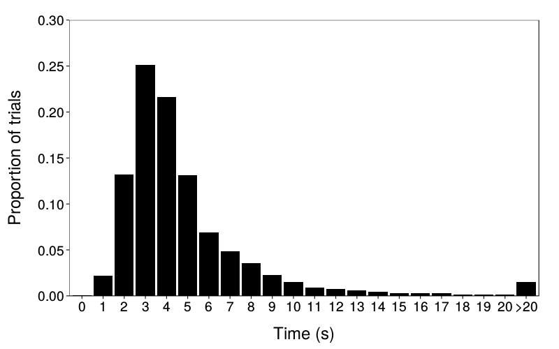
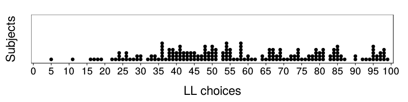
See Figure 1 for response times and Figure 2 for counts of LL choices.
Initial analysis
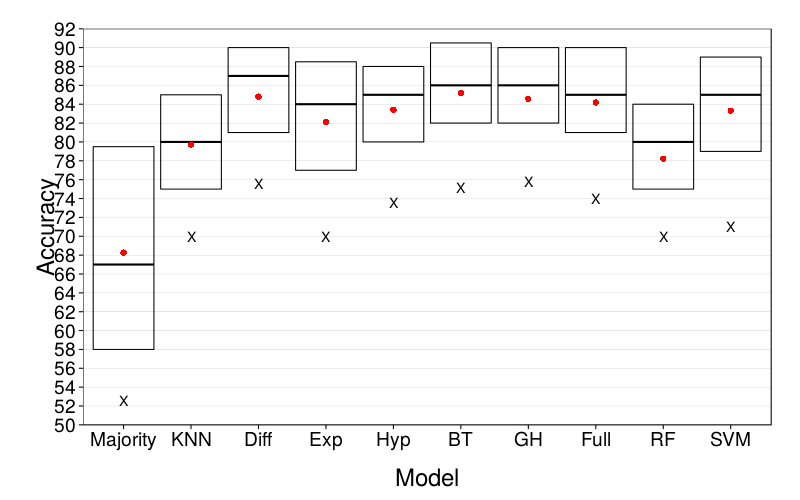
We first present cross-validated estimates of predictive accuracy, with no special treatment (such as shrinking or corruption) of the training data. As can be seen in Figure 3, all nontrivial models perform better than the trivial model Majority. The median accuracy (i.e., number of correct predictions) of Majority is 67, compared to 80 or more for all other models. Among the others, the overall picture is that KNN and RF lag behind the pack with medians of 80, while the remaining seven models perform similarly to each other with medians around 85. There is a suggestion that Exp and SVM do not handle difficult cases as well as the other well performing models, with bottom deciles near those of KNN and RF (around 70); however, far quantiles are necessarily estimated less precisely than medians.
Effect of training-set size
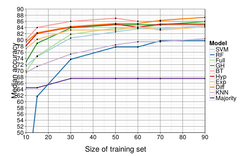
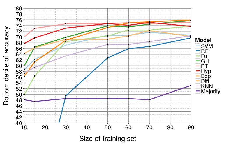
Figure 4 and Figure 5 show learning curves, that is, the effect of training-set size on predictive performance. Observe that most models' performance is not meaningfully affected until there are less than 50 training trials, far below the full set of 90. In fact, the best performers already have median accuracy 85 at a sample size of 30; since they fail to improve at higher sample sizes, we surmise that 85% accuracy is the approximate ceiling of median performance for this task.
RF flounders with small training sets, falling below Majority in performance as the training set grows smaller than 30 trials. KNN, as in the initial analysis, generally performs below average. Finally, at small sample sizes (15 and 10), the more complex GH, Full, and SVM begin to fall relative to the remaining four models by 5 to 10 choices. Otherwise, differences in model performance are again small.
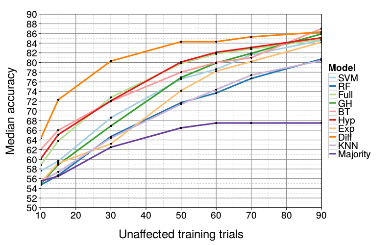
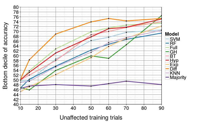
Effect of added noise
Figure 6 and Figure 7 show the effect of various degrees of corruption (setting training trials to SS or LL at random) on predictive performance. Clearly, all models are impaired by added noise; by the time only 10 of 90 training trials have been left intact, all bottom deciles are near 50% accuracy. In this analysis, we finally see a model with a clear advantage over all others: Diff is the most robust, showing a particular advantage when there is great but not overwhelming added noise. For example, at 50 intact trials, Diff's median (84) is still near ceiling whereas the best competitors have median 80. Only when there are more corrupted than intact training trials does Diff's performance meaningfully decrease from ceiling.
Of the remaining models, RF and KNN continue to underperform, and Exp, GH, and SVM become fragile at high levels of noise whereas Hyp, Full, and BT are slightly more robust, albeit not as robust as Diff.
Discussion
We compared how well 10 models could predict behavior in an intertemporal-choice task. We found that, given a generous amount of appropriate training data, most models considered within the intertemporal-choice literature perform above baseline but equally well. When only a little training data is available, more complex models begin to fall behind simpler models, but there is no clear winner among the simpler models. When noise is added to the training set, on the hand, we find that the difference model, a generalization of the arithmetic discounting of Doyle and Chen (2012), is particularly robust.
Perhaps the most notable aspect of our findings is the absence of meaningful differences between models. Extensive research of the kind cited earlier has investigated the explanatory merits of various models, and these theoretical differences are often stark, such as the exponential model's assumption that people are dynamically consistent and the hyperbolic model's assumption to the contrary. But we have found that these theoretical differences do not translate into meaningful differences in predictive power. Rather, what differences in predictive accuracy emerged in our analysis are most easily explained by statistical rather than psychological facts, like the disadvantage of more complex models at smaller sample sizes.
We know of one previous study that examined the predictive accuracy of intertemporal-choice models. Keller and Strazzera (2002) compared the cross-validated root mean square error of exponential and hyperbolic discounting models in a free-response task (p. 157). The hyperbolic model performed much better. In our study, by contrast, the hyperbolic model had at most a slight advantage over the exponential model. Possibly different kinds of models are most useful for prediction in free-response tasks than in forced-choice tasks. After all, given how the form of the dependent variable differs in these tasks (positive real numbers versus dichotomies), analogous models are required to take different forms anyway (e.g., we used logistic regression to transform continuous, real-valued preferences to discrete choices).
The difference model
What model should future researchers use to predict intertemporal choices? We think the difference model is a good choice. It is particularly simple, being a GLM using the difference between SS and LL along each dimension (delay and reward amount) as predictors. The logic here is parsimonious and easy to understand. As a GLM, the difference model is convenient to fit with software. In terms of accuracy, the difference model has the advantage of retaining its predictive accuracy when provided with very noisy training data. Thus, using the difference model could help to ameliorate data-quality concerns mundane and profound.
It is worth emphasizing that, in accordance with our interest in prediction over explanation, our findings in favor of the difference model are at most weak evidence that the difference model is how people actually make intertemporal decisions. Grace and McLean (2005) provide an example of evidence against the difference model as an explanation. Grace and McLean showed that presenting the LL reward as an increase over the SS reward (or vice versa) rather than as an absolute amount influenced subjects' choices. The difference model, using the difference between rewards as it does, cannot account for this finding. This finding is consistent with the theme long established by Kahneman and Tversky (e.g., Tversky & Kahneman, 1981) that normatively irrelevant presentation details must be considered to explain how people make decisions. It is an open question, however, whether modeling such details would improve our prediction of decisions.
Prediction versus explanation
Researchers often take it for granted that the models or theories that are most tenable as the explanation of a system—that best describe the data-generating process—are also the best at predicting the system's outputs. Our findings are a counterexample. Other such findings are not unheard of. In fact, it is possible for models with known-false assumptions to be more accurate than more realistic models. Domingos and Pazzani (1997) show that, even with simulated data generated from a known, complex model, a simpler model can perform better than the true model with realistic amounts of training data. Friedman (1953) wrote "theory is to be judged by its predictive power for the class of phenomena which it is intended to 'explain'", but also "Truly important and significant hypotheses will be found to have 'assumptions' that are wildly inaccurate descriptive representations of reality". In short, accuracy of description and accuracy of prediction are distinct, and to some extent antagonistic.
While research attempting to explain how people make decisions continues unabated, we hope to see more research on prediction of decisions. Keller and Strazzera (2002), discussed above, provides an illustration of how greatly test error can differ from training error due to overfitting. Glöckner and Pachur (2012) bring predictive analysis to the domain of risky decision-making.
Limitations and future directions
Our study had several limitations. First, our decision-making scenario was not incentive-compatible. That is, we did not give subjects financial motivation to answer our questions honestly. However, past studies have found little difference in subjects' intertemporal decision-making between tasks with real rewards and tasks with hypothetical rewards (e.g., Johnson & Bickel, 2002; Madden, Begotka, Raiff, & Kastern, 2003; Madden et al., 2004; Lagorio & Madden, 2005). Therefore, we believe that using real rewards would not have affected the results of our study.
Our philosophy in choosing the items for our binary-decision task was to be theoretically agnostic: we aimed for diversity over the representation of any theoretically relevant stimuli. Still, it is reasonable to ask how our results would have differed with different quartets. For example, only 21 of our 100 quartets had an immediate option (i.e., had an SS delay of 0). If immediate options had been represented more heavily, perhaps the models would have performed differently. Immediate outcomes are thought to have special importance (Mischel, Shoda, & Rodriguez, 1989); for example, the quasi-hyperbolic model (Laibson, 1997) treats delays of 0 differently from positive delays. Researchers may disagree as to which items are best, and it would not be clear how to reconcile different results obtained from studies with different items. The only real solution is to move out of the laboratory and examine external validity. After all, predicting behavior in laboratory tasks is only interesting insofar as laboratory behavior relates to real-life behavior. And it is unlikely that the distribution of quartets in a given real-life domain is uniform or otherwise has a neat structure of the kind one would use in basic research like our study. Ultimately, research on decisions about eating, spending, and drug use should use the model that can best predict the decisions of interest.
Although we have emphasized the ways in which explanatory and predictive goals can be at odds with each other, we hope that future research considers both. The differing, almost antagonistic perspectives of these goals mean they may actually serve complementary purposes in the comparison and refinement of models and theories.
References
Akaike, H. (1973). A new look at the statistical model identification. IEEE Transactions on Automatic Control, 19(6), 716–723. doi:10.1109/TAC.1974.1100705
Benhabib, J., Bisin, A., & Schotter, A. (2010). Present-bias, quasi-hyperbolic discounting, and fixed costs. Games and Economic Behavior, 69(2), 205–223. doi:10.1016/j.geb.2009.11.003
Bleichrodt, H., Potter van Loon, R. J. D., Rohde, K. I. M., & Wakker, P. P. (2013). A criticism of Doyle's survey of time preference: A correction regarding the CRDI and CADI families. Judgment and Decision Making, 8(5), 630–631. Retrieved from http://journal.sjdm.org/13/13723/jdm13723.html
Breiman, L. (2001). Random forests. Machine Learning, 45(1), 5–32.
Chung, S.-H., & Herrnstein, R. J. (1967). Choice and delay of reinforcement. Journal of the Experimental Analysis of Behavior, 10(1), 67–74. doi:10.1901/jeab.1967.10-67
Demurie, E., Roeyers, H., Baeyens, D., & Sonuga‐Barke, E. (2012). Temporal discounting of monetary rewards in children and adolescents with ADHD and autism spectrum disorders. Developmental Science, 15(6), 791–800. doi:10.1111/j.1467-7687.2012.01178.x
Domingos, P., & Pazzani, M. (1997). On the optimality of the simple Bayesian classifier under zero-one loss. Machine Learning, 29(1, 3), 103–130. doi:10.1023/A:1007413511361
Doyle, J. R. (2013). Survey of time preference, delay discounting models. Judgment and Decision Making, 8(2), 116–135. Retrieved from http://journal.sjdm.org/12/12309/jdm12309.html
Doyle, J. R., & Chen, C. H. (2012). The wages of waiting and simple models of delay discounting. doi:10.2139/ssrn.2008283
Friedman, M. (1953). The methodology of positive economics. In Essays in positive economics (pp. 3–43). Chicago, IL: University of Chicago Press.
Glöckner, A., & Pachur, T. (2012). Cognitive models of risky choice: Parameter stability and predictive accuracy of prospect theory. Cognition, 123(1), 21–32. doi:10.1016/j.cognition.2011.12.002
Grace, R. C., & McLean, A. P. (2005). Integrated versus segregated accounting and the magnitude effect in temporal discounting. Psychonomic Bulletin and Review, 12(4), 732–739. doi:10.3758/BF03196765
Green, L., Fristoe, N., & Myerson, J. (1994). Temporal discounting and preference reversals in choice between delayed outcomes. Psychonomic Bulletin and Review, 1(3), 383–389. doi:10.3758/BF03213979
Hastie, T., Tibshirani, R., & Friedman, J. H. (2009). The elements of statistical learning: Data mining, inference, and prediction (2nd ed.). New York, NY: Springer. Retrieved from http://www-stat.stanford.edu/~tibs/ElemStatLearn
Johnson, M. W., & Bickel, W. K. (2002). Within-subject comparison of real and hypothetical money rewards in delay discounting. Journal of the Experimental Analysis of Behavior, 77(2), 129–146. doi:10.1901/jeab.2002.77-129
Keller, L. R., & Strazzera, E. (2002). Examining predictive accuracy among discounting models. Journal of Risk and Uncertainty, 24(2), 143–160. doi:10.1023/A:1014067910173
Kirby, K. N., & Herrnstein, R. J. (1995). Preference reversals due to myopic discounting of delayed reward. Psychological Science, 6(2), 83–89. doi:10.1111/j.1467-9280.1995.tb00311.x
Kirby, K. N., & Maraković, N. N. (1995). Modeling myopic decisions: Evidence for hyperbolic delay-discounting within subjects and amounts. Organizational Behavior and Human Decision Processes, 64(1), 22–30. doi:10.1006/obhd.1995.1086
Koopmans, T. C. (1960). Stationary ordinal utility and impatience. Econometrica, 28(2), 287–309.
Lagorio, C. H., & Madden, G. J. (2005). Delay discounting of real and hypothetical rewards III: Steady-state assessments, forced-choice trials, and all real rewards. Behavioural Processes, 69(2), 173–187. doi:10.1016/j.beproc.2005.02.003
Laibson, D. (1997). Golden eggs and hyperbolic discounting. Quarterly Journal of Economics, 112(2), 443–477. doi:10.1162/003355397555253
Loewenstein, G., & Prelec, D. (1992). Anomalies in intertemporal choice: Evidence and an interpretation. Quarterly Journal of Economics, 107(2), 573–597. doi:10.2307/2118482
Luhmann, C. C. (2013). Discounting of delayed rewards is not hyperbolic. Journal of Experimental Psychology: Learning, Memory, and Cognition, 39(4), 1274–1279. doi:10.1037/a0031170
Luhmann, C. C., & Trimber, E. M. (2014). Fighting temptation: The relationship between executive control and self control. Submitted.
Madden, G. J., Begotka, A. M., Raiff, B. R., & Kastern, L. L. (2003). Delay discounting of real and hypothetical rewards. Experimental and Clinical Psychopharmacology, 11(2), 139–145. doi:10.1037/1064-1297.11.2.139
Madden, G. J., Bickel, W. K., & Jacobs, E. A. (1999). Discounting of delayed rewards in opioid-dependent outpatients: Exponential or hyperbolic discounting functions? Experimental and Clinical Psychopharmacology, 7(3), 284–293. doi:10.1037/1064-1297.7.3.284
Madden, G. J., Petry, N. M., Badger, G. J., & Bickel, W. K. (1997). Impulsive and self-control choices in opioid-dependent patients and non-drug-using control participants: Drug and monetary rewards. Experimental and Clinical Psychopharmacology, 5(3), 256–262. doi:10.1037/1064-1297.5.3.256
Madden, G. J., Raiff, B. R., Lagorio, C. H., Begotka, A. M., Mueller, A. M., Hehli, D. J., & Wegener, A. A. (2004). Delay discounting of potentially real and hypothetical rewards II: Between- and within-subject comparisons. Experimental and Clinical Psychopharmacology, 12(4), 251–261. doi:10.1037/1064-1297.12.4.251
Mazur, J. E. (1987). An adjusting procedure for studying delayed reinforcement. In M. L. Commons, J. E. Mazur, J. A. Nevin, & H. Rachlin (Eds.), The effect of delay and of intervening events on reinforcement value (pp. 55–73). Hillsdale, NJ: Lawrence Erlbaum. ISBN 0-89859-800-1.
McKerchar, T. L., Green, L., Myerson, J., Pickford, T. S., Hill, J. C., & Stout, S. C. (2009). A comparison of four models of delay discounting in humans. Behavioural Processes, 81(2), 256–259. doi:10.1016/j.beproc.2008.12.017
Meier, S., & Sprenger, C. D. (2010). Present-biased preferences and credit card borrowing. American Economic Journal: Applied Economics, 2(1), 193–210. doi:10.1257/app.2.1.193
Mischel, W., Shoda, Y., & Rodriguez, M. I. (1989). Delay of gratification in children. Science, 244(4907), 933–938. doi:10.1126/science.2658056
Myerson, J., & Green, L. (1995). Discounting of delayed rewards: Models of individual choice. Journal of the Experimental Analysis of Behavior, 64(3), 263–276. doi:10.1901/jeab.1995.64-263
Rachlin, H. (1995). Self-control: Beyond commitment. Behavioral and Brain Sciences, 18(1), 109–159. doi:10.1017/S0140525X00037602
Rachlin, H., & Green, L. (1972). Commitment, choice and self-control. Journal of the Experimental Analysis of Behavior, 17(1), 15–22. doi:10.1901/jeab.1972.17-15
Rissanen, J. (1978). Modeling by shortest data description. Automatica, 14(5), 465–471. doi:10.1016/0005-1098(78)90005-5
Rodriguez, M. L., & Logue, A. W. (1988). Adjusting delay to reinforcement: Comparing choice in pigeons and humans. Journal of Experimental Psychology: Animal Behavior Processes, 14(1), 105–117. doi:10.1037/0097-7403.14.1.105
Samuelson, P. A. (1937). A note on measurement of utility. Review of Economic Studies, 4(2), 155–161. doi:10.2307/2967612
Scholten, M., & Read, D. (2010). The psychology of intertemporal tradeoffs. Psychological Review, 117(3), 925–944. doi:10.1037/a0019619. Retrieved from http://repositorio.ispa.pt/bitstream/10400.12/580/1/rev-117-3-925.pdf
Scholten, M., & Read, D. (2013). Time and outcome framing in intertemporal tradeoffs. Journal of Experimental Psychology: Learning, Memory, and Cognition, 39(4), 1192–1212. doi:10.1037/a0031171
Schwarz, G. (1978). Estimating the dimension of a model. Annals of Statistics, 6(2), 461–464. doi:10.1214/aos/1176344136
Sutter, M., Kochaer, M. G., Rützler, D., & Trautmann, S. T. (2010). Impatience and uncertainty: Experimental decisions predict adolescents' field behavior (Discussion Paper No. 5404). Institute for the Study of Labor. Retrieved from http://ftp.iza.org/dp5404.pdf
Toubia, O., Johnson, E., Evgeniou, T., & Delquié, P. (2013). Dynamic experiments for estimating preferences: An adaptive method of eliciting time and risk parameters. Management Science, 59(3), 613–640. doi:10.1287/mnsc.1120.1570
Tversky, A., & Kahneman, D. (1973). Availability: A heuristic for judging frequency and probability. Cognitive Psychology, 5, 207–232. doi:10.1016/0010-0285(73)90033-9
Tversky, A., & Kahneman, D. (1981). The framing of decisions and the psychology of choice. Science, 211, 453–458. doi:10.1126/science.7455683
Vapnik, V. N. (2000). The nature of statistical learning theory (2nd ed.). New York, NY: Springer. ISBN 978-0-387-98780-4.
Varma, S., & Simon, R. (2006). Bias in error estimation when using cross-validation for model selection. BMC Bioinformatics, 7, 91. doi:10.1186/1471-2105-7-91