Cheat notebook
Created 14 Nov 2015 • Last modified 26 Jun 2018
Birthdates in voter data
- CA
- 1931-01-01: 17,195
- 1900-01-02 to 1901-01-01: each has 50 or more, compared to 1 to 1901-01-03
- FL
- 1942-10-10: 674, compared to 573 at most in the rest of the month
- KS
- 1901-01-01: 32, compared to 1s and 0s in the surrounding months
- NY
- 1901-01-01, 1950-01-01: 3,024 and 1,695, compared to less than 1,000 elsewhere
- 1921-01-01: 529, compared to at most 204 in the surrounding months
- OK
- There are 44 unique impossible dates: 19080000 19100000 19110000 19130000 19140000 19160000 19170000 19180000 19190000 19200000 19210000 19220000 19230000 19240000 19250000 19260000 19270000 19280000 19290000 19300000 19310000 19320000 19330000 19340000 19340931 19350000 19360000 19370000 19380000 19390000 19400000 19410000 19420000 19430000 19450000 19460100 19470000 19480000 19480014 19490000 19510000 19530000 19550000 19640000
AM and voter data
Descriptive
["Total voters" (format (.sum ($ counts voters)) ",")]
| Total voters | 48,852,975 |
Match rate:
(setv statecounts (.sum (.groupby
  (getl counts : (qw state voters am_users)) "state")))
(setv state-summary (apply cbind (rmap [state (filt (in it am-users-in-states) states)]
  (setv matched (int (getl statecounts state "am_users")))
  (setv total-am (get am-users-in-states state))
  (setv voters (int (getl statecounts state "voters")))
  (setv pop (get state-pop-2012 state))
  (setv party-counts (do
    (setv d (ss counts (= $state state)))
    (setv [pv vv] (map second (.iteritems (getl d : (qw party voters)))))
    (setv pv (.set-categories pv.cat (+ keep-parties ["rest"])))
    (setv pv (.fillna pv "rest"))
    (setv d (.sum (.groupby (cbind pv vv) 0)))
    (list (.iteritems (geti d : 0)))))
  (pds-from-pairs :name (get state-names state) (+ party-counts (pairs
      "Total registered voters" voters
      "Population" pop
      "Percent covered" (round (* 100 (/ voters pop)))
      "AM users matched with voters" matched
      "Total AM users" total-am
      "Percent matched" (round (* 100 (/ matched total-am)))))))))
(setv state-summary.index.name "State")
(setv state-summary (.fillna state-summary 0))
(setv state-summary (.applymap state-summary (λ (format (int it) ","))))
(.rename state-summary :inplace T :index {
  "np" "Unaffiliated voters"
  "DEM" "Democrats"
  "REP" "Republicans"
  "GRE" "Greens"
  "LBT" "Libertarians"
  "rest" "Voters in other party"})
state-summary
| State | California | Florida | Kansas | New York | Oklahoma |
|---|---|---|---|---|---|
| Unaffiliated voters | 2,710,719 | 2,700,397 | 522,094 | 3,016,645 | 229,494 |
| Democrats | 7,936,325 | 4,988,433 | 432,858 | 7,134,846 | 879,343 |
| Republicans | 5,297,443 | 4,378,861 | 773,346 | 3,484,717 | 844,305 |
| Greens | 114,126 | 6,143 | 0 | 32,811 | 0 |
| Libertarians | 110,808 | 12,016 | 11,690 | 4,710 | 0 |
| Voters in other party | 2,004,915 | 429,399 | 0 | 796,528 | 3 |
| Total registered voters | 18,174,336 | 12,515,249 | 1,739,988 | 14,470,257 | 1,953,145 |
| Population | 38,041,430 | 19,317,568 | 2,885,905 | 19,570,261 | 3,814,820 |
| Percent covered | 48 | 65 | 60 | 74 | 51 |
| AM users matched with voters | 32,457 | 17,928 | 2,642 | 21,776 | 2,072 |
| Total AM users | 92,058 | 43,987 | 6,282 | 54,203 | 6,603 |
| Percent matched | 35 | 41 | 42 | 40 | 31 |
Match rates range from 31% to 42%.
Here's a breakdown of gender and gender imputation.
(setv d (.reset-index (.applymap
  (.dropna (.sum (.groupby
    (.replace (getl counts : (qw state gender_known gender voters)) np.nan "Unknown")
    (qw state gender_known gender))))
  (λ (format (int it) ",")))))
(.sort-values d (qw state gender_known gender)
  :ascending [True False True])
| I | state | gender_known | gender | voters |
|---|---|---|---|---|
| 3 | CA | True | Female | 6,279,902 |
| 4 | CA | True | Male | 5,453,470 |
| 0 | CA | False | Female | 2,991,313 |
| 1 | CA | False | Male | 2,617,152 |
| 2 | CA | False | Unknown | 832,499 |
| 8 | FL | True | Female | 6,641,276 |
| 9 | FL | True | Male | 5,645,059 |
| 5 | FL | False | Female | 97,195 |
| 6 | FL | False | Male | 94,095 |
| 7 | FL | False | Unknown | 37,624 |
| 13 | KS | True | Female | 921,923 |
| 14 | KS | True | Male | 817,735 |
| 10 | KS | False | Female | 132 |
| 11 | KS | False | Male | 122 |
| 12 | KS | False | Unknown | 76 |
| 18 | NY | True | Female | 7,909,124 |
| 19 | NY | True | Male | 6,560,341 |
| 15 | NY | False | Female | 298 |
| 16 | NY | False | Male | 285 |
| 17 | NY | False | Unknown | 209 |
| 20 | OK | False | Female | 938,158 |
| 21 | OK | False | Male | 777,237 |
| 22 | OK | False | Unknown | 237,750 |
The OK voter data has no gender information, so we had to impute every case there.
(setv n-total (.sum ($ counts voters)))
(setv n-not-given (.sum ($ (ss counts (~ $gender_known)) voters)))
(setv n-imputed (.sum ($
  (ss counts (& (.notnull $gender) (~ $gender_known)))
  voters)))
(rd [
  ["Proportion of genders missing" (/ n-not-given n-total)]
  ["Proprtion of missing genders imputed" (/ n-imputed n-not-given)]
  ["Proportion of genders still missing" (/ (- n-not-given n-imputed) n-total)]])
| Proportion of genders missing | 0.177 |
| Proprtion of missing genders imputed | 0.872 |
| Proportion of genders still missing | 0.023 |
(setv n-bad-age (.sum ($ (ss counts (.isnull $age)) voters)))
["Proportion of ages invalid" (format (/ n-bad-age n-total) ".03f")]
| Proportion of ages invalid | 0.010 |
Here is the number of registered voters per party and state (ignoring the AM data).
(setv x (.sort-values
  (.reset-index
    (.sum ($ (.set-index counts ["state" "party"]) voters)
      :level ["state" "party"]))
  ["state" "voters"]
  :ascending [True False]))
(setv ($ x voters) (amap (.format "{:,}" it) ($ x voters)))
(setv x (.reset-index :drop T x))
x
| I | state | party | voters |
|---|---|---|---|
| 0 | CA | DEM | 7,936,325 |
| 1 | CA | REP | 5,297,443 |
| 2 | CA | np | 2,710,719 |
| 3 | CA | DS | 1,114,635 |
| 4 | CA | AI | 479,378 |
| 5 | CA | OTH | 271,806 |
| 6 | CA | GRE | 114,126 |
| 7 | CA | LBT | 110,808 |
| 8 | CA | PF | 63,014 |
| 9 | CA | MIS | 61,684 |
| 10 | CA | REF | 7,786 |
| 11 | CA | AME | 3,379 |
| 12 | CA | NAT | 2,271 |
| 13 | CA | WWP | 313 |
| 14 | CA | JP | 146 |
| 15 | CA | CTP | 113 |
| 16 | CA | CPC | 96 |
| 17 | CA | WP | 50 |
| 18 | CA | PIR | 31 |
| 19 | CA | CP | 31 |
| 20 | CA | CMP | 31 |
| 21 | CA | HUM | 27 |
| 22 | CA | HPC | 14 |
| 23 | CA | MMW | 11 |
| 24 | CA | OP | 9 |
| 25 | CA | PPC | 9 |
| 26 | CA | NRP | 8 |
| 27 | CA | TVP | 7 |
| 28 | CA | ACP | 7 |
| 29 | CA | UCA | 6 |
| 30 | CA | MCP | 4 |
| 31 | CA | FED | 4 |
| 32 | CA | NMB | 4 |
| 33 | CA | DP | 4 |
| 34 | CA | AMC | 4 |
| 35 | CA | SEU | 4 |
| 36 | CA | WFP | 4 |
| 37 | CA | SAP | 3 |
| 38 | CA | LRU | 3 |
| 39 | CA | CPP | 3 |
| 40 | CA | EJP | 3 |
| 41 | CA | POT | 2 |
| 42 | CA | GSP | 2 |
| 43 | CA | EGA | 2 |
| 44 | CA | UMP | 2 |
| 45 | CA | APP | 1 |
| 46 | CA | UCB | 1 |
| 47 | CA | NSP | 1 |
| 48 | CA | U08 | 1 |
| 49 | CA | ATP | 1 |
| 50 | FL | DEM | 4,988,433 |
| 51 | FL | REP | 4,378,861 |
| 52 | FL | np | 2,700,397 |
| 53 | FL | INT | 280,485 |
| 54 | FL | UNK | 59,740 |
| 55 | FL | IDP | 58,517 |
| 56 | FL | NRS | 25,928 |
| 57 | FL | LBT | 12,016 |
| 58 | FL | GRE | 6,143 |
| 59 | FL | REF | 2,037 |
| 60 | FL | CPF | 1,119 |
| 61 | FL | AIP | 452 |
| 62 | FL | TPF | 391 |
| 63 | FL | FPP | 336 |
| 64 | FL | ECO | 166 |
| 65 | FL | PSL | 122 |
| 66 | FL | PFP | 45 |
| 67 | FL | FSW | 29 |
| 68 | FL | JPF | 12 |
| 69 | FL | OBJ | 12 |
| 70 | FL | AEL | 4 |
| 71 | FL | FWP | 3 |
| 72 | FL | SOC | 1 |
| 73 | KS | REP | 773,346 |
| 74 | KS | np | 522,094 |
| 75 | KS | DEM | 432,858 |
| 76 | KS | LBT | 11,690 |
| 77 | NY | DEM | 7,134,846 |
| 78 | NY | REP | 3,484,717 |
| 79 | NY | np | 3,016,645 |
| 80 | NY | IND | 557,885 |
| 81 | NY | CON | 183,041 |
| 82 | NY | WOR | 55,420 |
| 83 | NY | GRE | 32,811 |
| 84 | NY | LBT | 4,710 |
| 85 | NY | FDM | 110 |
| 86 | NY | RTH | 58 |
| 87 | NY | TXP | 6 |
| 88 | NY | APP | 5 |
| 89 | NY | SWP | 3 |
| 90 | OK | DEM | 879,343 |
| 91 | OK | REP | 844,305 |
| 92 | OK | np | 229,494 |
| 93 | OK | AE | 3 |
Florida and California have quite a few voters with undocumented party codes.
The web page for New York's Independence Party states that "The Party's leadership recognizes that individuals do sometimes unwittingly register as members of the Independence Party when their intent was to register to vote as a 'blank'." That may explain why CA, FL, and NY all have so many people in an "Independence Party" or "Independent Party" when I've never even heard of such a party before. Here's the number of people in each such party:
(ss x (.isin $party (qw IND IDP INT AI)))
| I | state | party | voters |
|---|---|---|---|
| 4 | CA | AI | 479,378 |
| 53 | FL | INT | 280,485 |
| 55 | FL | IDP | 58,517 |
| 80 | NY | IND | 557,885 |
Below, voters shows the number of registered voters for each state and party, and AMr shows the reciprocal of the Ashley Madison match rate (e.g., 500 means that 1 in 500 such voters were matched to an Ashley Madison user).
(setv x (.dropna (.sum (.groupby
  (getl (drop-unused-cats (ss counts (.isin $party keep-parties)))
    : (qw state party voters am_users))
  (qw state party)))))
(setv ($ x AMr) (wc x (/ $voters $am_users)))
(setv x (.drop x "am_users" 1))
(setv xR (.reset-index x))
(setv ($ xR state) (.map ($ xR state) state-names))
(.to-csv xR "/tmp/amr.csv")
(.applymap x (λ (if (numeric? it) (format (int (round it)) ",") it)))
| state | party | voters | AMr |
|---|---|---|---|
| CA | np | 2,710,719 | 527 |
| CA | DEM | 7,936,325 | 703 |
| CA | REP | 5,297,443 | 476 |
| CA | GRE | 114,126 | 399 |
| CA | LBT | 110,808 | 260 |
| FL | np | 2,700,397 | 629 |
| FL | DEM | 4,988,433 | 1,057 |
| FL | REP | 4,378,861 | 542 |
| FL | GRE | 6,143 | 410 |
| FL | LBT | 12,016 | 300 |
| KS | np | 522,094 | 587 |
| KS | DEM | 432,858 | 1,007 |
| KS | REP | 773,346 | 604 |
| KS | LBT | 11,690 | 285 |
| NY | np | 3,016,645 | 627 |
| NY | DEM | 7,134,846 | 901 |
| NY | REP | 3,484,717 | 485 |
| NY | GRE | 32,811 | 566 |
| NY | LBT | 4,710 | 236 |
| OK | np | 229,494 | 702 |
| OK | DEM | 879,343 | 1,573 |
| OK | REP | 844,305 | 712 |
Here's a plot. (The y-axis is upside-down so that higher points mean more Ashley Madison users.)
library(ggplot2)

d = read.csv("/tmp/amr.csv")
d = transform(d, party = factor(party, levels =
    c("np", "DEM", "REP", "GRE", "LBT")))
breaks = c(1, seq(250, 1750, 250))
amr.plot = ggplot(d) +
    geom_point(aes(state, AMr)) +
    geom_text(aes(
        x = as.integer(state) + ifelse(party == "REP", -.05, .05),
        y = AMr,
        label = c(
            np = "none", DEM = "Dem", REP = "Rep",
            GRE = "Green", LBT = "Lib")[as.character(party)],
        hjust = ifelse(party == "REP", 1, 0))) +
    xlab("State") +
    scale_y_reverse(name = "Ashley Madison users",
      expand = c(0, 0),
      breaks = breaks,
      labels = paste("1 in", formatC(breaks, big.mark = ","))) +
    coord_cartesian(ylim = range(breaks)) +
    theme(
        panel.grid.major = element_blank(),
        panel.grid.minor = element_blank(),
        panel.border = element_blank(),
        axis.text.x = element_text(color = "black"),
        axis.text.y = element_text(color = "black"),
        axis.line = element_line(color = "black"))
amr.plot
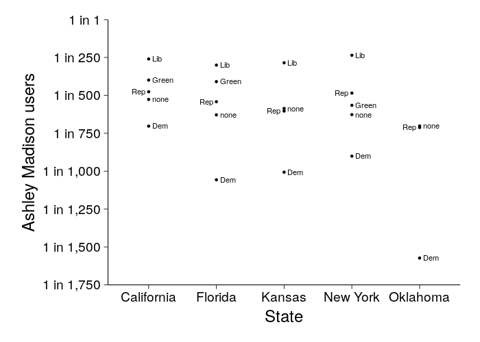
In all five states, Dems cheat less than other party categories (including the more liberal Greens). In all four states with a libertarian party, libertarians cheat more than other party categories.
Here are the AM rates by state alone:
(setv x (getl (.sum (.groupby counts "state")) : (qw voters am_users)))
(setv ($ x AMr) (wc x (/ $voters $am_users)))
;(setv x (.drop x "am_users" 1))
;(setv xR (.reset-index x))
;(setv ($ xR state) (.map ($ xR state) state-names))
;(.to-csv xR "/tmp/amr.csv")
(ordf (.applymap x (λ (if (numeric? it) (format (int (round it)) ",") it)))
  $AMr)
| state | voters | am_users | AMr |
|---|---|---|---|
| CA | 18,174,336 | 32,457 | 560 |
| KS | 1,739,988 | 2,642 | 659 |
| NY | 14,470,257 | 21,776 | 665 |
| FL | 12,515,249 | 17,928 | 698 |
| OK | 1,953,145 | 2,072 | 943 |
Party membership differs by gender and age. If we consider only males, and we control for age, do we still see these AM usage differences by party? Below is a crude graph where we group men by year of birth.
(setv cs (getl
  (ss counts
    (& (= $gender "Male") (.notnull $born)
      (.isin $party ["np" "DEM" "REP"])))
  :
  (qw state born party am n)))
(setv out (.dropna (.apply
  (.groupby cs ["state" (// ($ cs born) 10000) "party"])
  (λ (if (.any ($ it am))
    (/ (.sum ($ (ss it [[var:a]][[var:m]]) [[var:n]])) (.[[var:s]][[var:u]][[var:m]] ( it n)))
    0)))))
(setv out (kwc pd.DataFrame out :columns ["am_proportion"]))
;(pd.Series [(.sum ($ it n)) (.sum ($ (ss it $am) n))] ["n" "a"])))))
(.to-csv out "/tmp/am-year-party.csv")
d = read.csv("/tmp/am-year-party.csv")
library(ggplot2)
ggplot(subset(d, born >= 1915)) +
   geom_line(aes(born, am_proportion, color = party)) +
   scale_color_manual(values = c("blue", "darkgreen", "red")) +
   facet_grid(state ~ ., scales = "free")
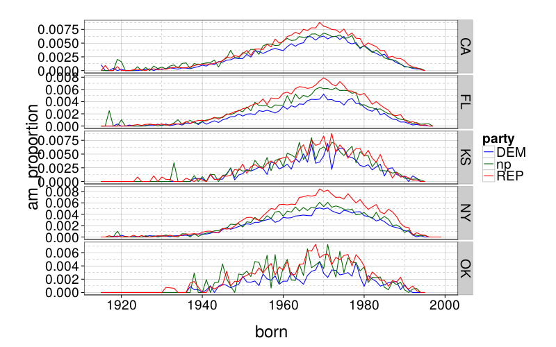
It looks like it, pretty much.
Modeling
Basic information about the data we'll use for modeling:
(setv d (am-usage-filter counts))
(setv base-rate (/ (.sum ($ d am_users)) (.sum ($ d voters))))
[
  ["Sample size" (format (.sum ($ d voters)) ",")]
  ["AM users"    (format (.sum ($ d am_users)) ",")]
  ["Base rate" (+ "1 in " (str (int (round (/ 1 base-rate)))))]
  ["Base MSE" (round (* base-rate (- 1 base-rate)) 8)]]
| Sample size | 44,172,769 |
| AM users | 69,023 |
| Base rate | 1 in 640 |
| Base MSE | 0.00156013 |
(setv folds (do
  (setv old-rng-state (np.random.get-state))
  (np.random.seed 55)
  (setv out (gen-counts-cv-folds-ts ($ d voters) ($ d am_users) 10))
  (np.random.set-state old-rng-state)
  out))

(import [collections [OrderedDict]])

(setv models (OrderedDict (,
  [:Trivial {:desc "No predictors" :formula
    None}]
  [:Parties {:desc "Predictors: party only" :formula
    "party"}]
  [:Demo {:desc "Predictors: state, gender, age" :formula
    "state + female + age + age2"}]
  [:DemoParties {:desc "Predictors: state, gender, age, party" :formula
    "state + female + age + age2 + party"}]
  [:IntDemo {:desc "Demo, plus all first-order interactions" :formula (.join " " [
    "state + female + age + age2 +"
    "female:(state + age + age2) +"
    "state:(age + age2)"])}]
  [:IntDemoParties {:desc "DemoParties, plus all first-order interactions" :formula (.join " " [
    "state + female + age + age2 + party +"
    "female:(state + age + age2 + party) +"
    "state:(age + age2 + party) +"
    "party:(age + age2)"])}])))
(for [[k v] (.items models)]
  (setv (get v :name) (keyword->str k)))

(for [model (.values models)]
  (.update model (cached-eval
    (+ "am-usage-cv " (get model :name))
    :cache-dir cache-dir
    (fn []
      (if (= (get model :name) "Trivial")
        (am-usage "cv" counts "state" folds :trivial-model T)
        (am-usage "cv" counts (get model :formula) folds))))))

(setv cv-results (df-from-pairs (rmap [model (.values models)] (pairs
  "Model" (get model :name)
  "Description" (get model :desc)
  "Terms" (if (= (get model :name) "Trivial") 1
    (+ 1 (len (get model :x-column-names))))
  "MSE" (round (get model :cv-mse) 9)
  "[[var:p]]_{0}" (.format "^{}" (int (round (/ 1 (get model :cv-p-cond 0)))))
  "[[var:p]]_{1}" (.format "^{}" (int (round (/ 1 (get model :cv-p-cond 1)))))))))
(setv cv-results (.set-index cv-results "Model"))
cv-results
| Model | Description | Terms | MSE | p0 | p1 |
|---|---|---|---|---|---|
| Trivial | No predictors | 1 | 0.001560127 | ^640 | ^640 |
| Parties | Predictors: party only | 5 | 0.001559982 | ^640 | ^604 |
| Demo | Predictors: state, gender, age | 8 | 0.001555791 | ^642 | ^232 |
| DemoParties | Predictors: state, gender, age, party | 12 | 0.001555600 | ^642 | ^226 |
| IntDemo | Demo, plus all first-order interactions | 22 | 0.001555783 | ^642 | ^231 |
| IntDemoParties | DemoParties, plus all first-order interactions | 51 | 0.001555565 | ^642 | ^224 |
Here p0 is the reciprocal of the mean predicted probability among all voters who didn't actually use AM, and p1 is the same thing for voters who actually did use AM.
None of the models can improve much on the base rate for p0. parties_only somewhat improves p1, while all the other nontrivial models substantially improve p1. Parties help, and interaction terms help a tiny bit more.
Below are the coefficients of the parties and ints&parties models.
(setv noint-coefs (cache
  (am-usage "fit_all" counts :formula
    (get models :DemoParties :formula))))
(setv int-coefs (cache
  (am-usage "fit_all" counts :formula
    (get models :IntDemoParties :formula))))

(defn pretty-term-name [s] (cond
  [(in ":" s) (do
    (setv [s1 s2] (.split s ":"))
    (+ (pretty-term-name s1) " × " (pretty-term-name s2)))]
  [(= s "age")
    "Age"]
  [(= s "age2")
    "Age²"]
  [(= s "female[T.True]")
    "Female"]
  [(.startswith s "state[")
    (.format "State: {}" (get state-names (cut (.rstrip s "]") -2)))]
  [(.startswith s "party[")
    (.format "Party: {}" (get long-party-names (cut (.rstrip s "]") -3)))]
  [True
    s]))

(setv pretty-coefs (.applymap
  (cbind :DemoParties noint-coefs :IntDemoParties int-coefs)
  (λ (if (np.isnan it) "" (.replace (format it ".02f") "-" "−")))))
(setv pretty-coefs.index (amap (pretty-term-name it) pretty-coefs.index))
(setv pretty-coefs.index.name "Term")
pretty-coefs
| Term | DemoParties | IntDemoParties |
|---|---|---|
| Intercept | −6.20 | −6.22 |
| Age | −1.07 | −1.10 |
| Age² | −2.23 | −2.14 |
| Female | −3.31 | −3.13 |
| Female × Age | 0.52 | |
| Female × Age² | 0.43 | |
| Female × Party: Democratic | 0.18 | |
| Female × Party: Green | −0.08 | |
| Female × Party: Libertarian | 0.03 | |
| Female × Party: Republican | −0.01 | |
| Female × State: California | −0.14 | |
| Female × State: Florida | −0.14 | |
| Female × State: Kansas | −0.23 | |
| Female × State: Oklahoma | −0.23 | |
| Party: Democratic | −0.18 | −0.17 |
| Party: Democratic × Age | −0.13 | |
| Party: Democratic × Age² | 0.08 | |
| Party: Green | 0.02 | −0.19 |
| Party: Green × Age | 0.22 | |
| Party: Green × Age² | −0.29 | |
| Party: Libertarian | 0.46 | 0.47 |
| Party: Libertarian × Age | −0.34 | |
| Party: Libertarian × Age² | −0.34 | |
| Party: Republican | 0.19 | 0.28 |
| Party: Republican × Age | −0.21 | |
| Party: Republican × Age² | 0.05 | |
| State: California | 0.14 | 0.16 |
| State: California × Age | 0.22 | |
| State: California × Age² | −0.19 | |
| State: California × Party: Democratic | 0.06 | |
| State: California × Party: Green | 0.23 | |
| State: California × Party: Libertarian | −0.15 | |
| State: California × Party: Republican | −0.16 | |
| State: Florida | −0.04 | 0.01 |
| State: Florida × Age | 0.19 | |
| State: Florida × Age² | −0.22 | |
| State: Florida × Party: Democratic | −0.13 | |
| State: Florida × Party: Green | 0.42 | |
| State: Florida × Party: Libertarian | −0.25 | |
| State: Florida × Party: Republican | −0.10 | |
| State: Kansas | −0.10 | −0.16 |
| State: Kansas × Age | −0.33 | |
| State: Kansas × Age² | −0.59 | |
| State: Kansas × Party: Democratic | −0.07 | |
| State: Kansas × Party: Libertarian | −0.08 | |
| State: Kansas × Party: Republican | −0.25 | |
| State: Oklahoma | −0.31 | −0.15 |
| State: Oklahoma × Age | 0.23 | |
| State: Oklahoma × Age² | −0.14 | |
| State: Oklahoma × Party: Democratic | −0.26 | |
| State: Oklahoma × Party: Republican | −0.20 |
Let's make predictions for a 40-year-old male New Yorker.
Using the parties model:
(setv [age-t age2-t] (am-usage-transform-ages
  (am-usage-filter counts) 40))
(defn f [coefs]
  (defn c [k] (.get coefs k 0))
  (setv l (lc [[name v] (+ [["party[T.np]" 0]] (list (.iteritems coefs)))]
    (re.match r"party\[T\.[A-Za-z]+\]\Z" name)
    (, (.group (re.search "T.([A-Za-z]+)" name) 1) (int (round (/ 1 (ilogit (+
      (get noint-coefs "Intercept")
      (* age-t (c "age"))
      (* age2-t (c "age2"))
      (* age-t (c (+ name ":age")))
      (* age2-t (c (+ name ":age2")))
      v))))))))
  (geti (.set-index (pd.DataFrame l) 0) : 0))
(.sort-values (f noint-coefs))
| I | 1 |
|---|---|
| LBT | 117 |
| REP | 152 |
| GRE | 180 |
| np | 184 |
| DEM | 219 |
Using the ints_and_parties model:
(setv predcompare (cbind :DemoParties (f noint-coefs) :IntDemoParties (f int-coefs)))
(setv predcompare (.applymap (.sort-values predcompare "DemoParties")
  (λ (.format "^{}" it))))
(setv predcompare.index (amap (get long-party-names it) predcompare.index))
(setv predcompare.index.name "Party")
predcompare
| Party | DemoParties | IntDemoParties |
|---|---|---|
| Libertarian | ^117 | ^98 |
| Republican | ^152 | ^138 |
| Green | ^180 | ^219 |
| unaffiliated | ^184 | ^189 |
| Democratic | ^219 | ^223 |
Old modeling (with SGD)
Would it make things substantially easier if all IVs were discrete? Potentially, yes, since when all IVs of a logistic-regression model are discrete, and all interaction terms are included (and there's no regularization or anything else special), the best-fitting logistic-regression model just reproduces the contingency table. However, the cells of the IV contingency table here vary widely in size. Some are 0, because, e.g., I don't have data for Greens in Kansas.
SGDClassifier can do probabilistic prediction not only with logistic loss (which is what I've done) but also with modified Huber loss. However, I bet it would be less effective.
(setv [n-modeling-subjects n-modeling-cheated] (cache (get-modeling-ns)))
(setv base-rate (/ n-modeling-cheated n-modeling-subjects))
[
  ["Sample size" (format n-modeling-subjects ",")]
  ["Cheated" (format n-modeling-cheated ",")]
  ["Base rate" (+ "1 in " (str (int (/ 1 base-rate))))]
  ["Base MSE" (round (* base-rate (- 1 base-rate)) 8)]]
| Sample size | 45,201,799 |
| Cheated | 68,602 |
| Base rate | 1 in 658 |
| Base MSE | 0.00151538 |
(setv cv-results (dict (cache (lc [ii [False True] ipp [False True]]
  (, (, ii ipp) (kwc try-model "cv" n-modeling-subjects n-modeling-cheated
    :include-interactions ii
    :include-party-params ipp))))))
(kwc .set-index :keys "model" (kwc pd.DataFrame :columns ["model" "MSE" "P when 0" "P when 1"] (+
  [["trivial" (round (* base-rate (- 1 base-rate)) 8)
    (int (/ 1 base-rate)) (int (/ 1 base-rate))]]
  (lc [ii [False True] ipp [False True]] [
      (.format "{}, {}"
        (if ii "interacts" "no interacts")
        (if ipp "parties" "no parties"))
      (round (get cv-results (, ii ipp) "mse") 8)
      (int (/ 1 (get cv-results (, ii ipp) "mean pred prob when 0")))
      (int (/ 1 (get cv-results (, ii ipp) "mean pred prob when 1")))]))))
| model | MSE | P when 0 | P when 1 |
|---|---|---|---|
| trivial | 0.00151538 | 658 | 658 |
| no interacts, no parties | 0.00139625 | 709 | 333 |
| no interacts, parties | 0.00139611 | 724 | 330 |
| interacts, no parties | 0.00139643 | 706 | 375 |
| interacts, parties | 0.00139615 | 719 | 351 |
Here we compared the fivefold cross-validate performance of four models, and also include base rates for comparison. The rightmost two columns give the mean predicted probability of cheating (expressed as a reciprocal) among subjects who were not (0) or were (1) actually cheating. We see that all models improve substantially upon the base rate, and adding party terms helps, but interactions don't help. So let's use the model with parties but no interactions.
Here are its parameters with fit to the whole dataset:
(setv params (OrderedDict (cache (kwc try-model "fit" n-modeling-subjects n-modeling-cheated
  :!include-interactions :+include-party-params))))
(lc [[name value] (.items params)] [name (rd value)])
| Intercept | -5.106 |
| CA | 0.064 |
| FL | -0.196 |
| KS | -0.247 |
| OK | -0.430 |
| known_female | -3.226 |
| unknown_gender | -0.934 |
| age | -1.059 |
| age_squared | -0.978 |
| DEM | -0.198 |
| REP | 0.191 |
| GRE | -0.044 |
| LBT | 0.085 |
We can use them to create a little table of the predicted probability of a 25-year-old male New Yorker cheating:
(defn p [x] (get params x))
(kwc sorted :key second (lc [party keep-parties]
  (, party (int (/ 1 (ilogit (+
    (p "Intercept")
    ;(p "NY")
    (* (p "age") (first (transformed-age 25)))
    (* (p "age_squared") (second (transformed-age 25)))
    (if (= party "np") 0 (p party)))))))))
| REP | 182 |
| LBT | 202 |
| np | 220 |
| GRE | 230 |
| DEM | 268 |
We see that Democrats have the lowest probability of cheating, but differently from the simple graph above, Greens and libertarians are between Republicans and Democrats rather than cheating more than Republicans. The differences here are generally much smaller than those in the graph; the biggest difference is between Republicans and Democrats, which has Democrats cheat about a third less than Republicans.
Matching voter records across years
First attempt
As a test run, we consider NY 2010 and 2012. I compute how many records each dataset has that the other doesn't have by just subtracting the number of shared records.
- Matching by
rn- 2010: 13,026,768 records
- 2012: 14,500,804 records
- Shared: 13,017,759
- 2010-only records: 9,009
- 2012-only records: 1,483,045
- Matching by
name,zip,addrnum1,addrnum2- 2010: 12,852,502 distinct records
- 2012: 14,283,937 distinct records
- Shared: 10,854,796
- 2010-only records: 1,997,706
- 2012-only records: 3,429,141
Matching by rn, 1,385,648 of the pairs of records have a different addrnum1 or addrnum2.
Matching by rn, 12,999,937 of the 13,017,473 (99.87%) pairs of records have matching birthdates.
2010 voters matched to AM: 20,191
- By
rn, 20,171 of these are also present in 2012. - And 1,803 have a new
addrnum1oraddrnum2.sqlite3 voter.sqlite 'attach "voter-2010.sqlite" as V10; select count(*) from (select rn, addrnum1, addrnum2 from V10.T where am_user notnull) as T10 join T as T12 using (rn) where T10.addrnum1 != T12.addrnum1 or T10.addrnum2 != T12.addrnum2
- 1,803 / 20,171 = .09
2010 voters not matched to AM:
- By
rn, 12,997,588 are present in 2012. - And 1,383,845 of those have a new
addrnum1oraddrnum2. - 1,383,845 / 12,997,588 = .11
Notice that this difference is in the wrong direction: 2010 New York voters were slightly less likely to have a different address in 2012 if they were on AM.
We might do this better by handling time more explicitly on both sides, using transaction dates to date AM usage and record modification dates (when they exist) to date voter records.
Using transaction dates
I hoped to use registration dates as an indicator of when each voter record was last updated. However, this doesn't seem to be correct, at least for New York, because sqlite3 voter.sqlite 'attach "voter-2010.sqlite" as V10; select V10.T.registered < V12T.registered as updated, V10.T.addrnum1 != V12T.addrnum1 as moved, count(*) from (T as V12T inner join V10.T using (rn)) group by updated, moved returns:
| 0 | 0 | 11639406 |
| 0 | 1 | 1076701 |
| 1 | 0 | 11582 |
| 1 | 1 | 289784 |
which shows us that quite a few seemingly non-updated 2012 records have new addresses. So instead, let's just use January 1st, 2012, as the threshold date. (Or rather, January 3rd, to provide some wiggle room for time-zone shenanigans.)
attach "voter-2010.sqlite" as V10;
attach "amcc.sqlite" as AMCC;
select
  V12T.am_user notnull and early_enough as am_before,
  V12T.addrnum1 != V10.T.addrnum1 as moved,
  count(*)
  from (T as V12T inner join V10.T using (rn))
      left outer join (select
         usernum,
         min(time) < cast(strftime("%s", "20120103") as integer)
             as early_enough
--         cast(strftime("%Y%m%d", min(time) - 2*24*60*60, "unixepoch", "utc") as integer)
--             as first_am
         from AMCC.T
         group by usernum)
      on V12T.am_user = usernum
  where V12T.am_user isnull or V12T.am_user != -1
  group by am_before, moved;
| 0 | 0 | 11632713 |
| 0 | 1 | 1363900 |
| 1 | 0 | 16329 |
| 1 | 1 | 2337 |
- Among moved, 2337 / 1363900 = 1 / 584 used AM before 2012
- Among non-moved, 16329 / 11632713 = 1 / 712 used AM before 2012
- Among AM users before 2012, 2337 / 16329 = 14% moved
- Among non-AM users before 2012, 1363900 / 11632713 = 12% moved
That's in the right direction, at least.
I'm still matching up AM users with voters using 2012 voter addresses. Should I be using the 2010 voter addresses instead? Should I use both somehow?
Diversity of names in voter data
One odd explanation I thought of for the finding that Republicans use AM more than Democrats is that Republicans may have less variety in full names (i.e., combination of first name and last name), inflating the number of false positives. In particular, Republicans being whiter than Democrats suggests there should be a smaller pool of names.
The 2012 voter records have 21,371,805 Democrats and 14,778,672 Republicans.
> sqlite3 ../data/voter.sqlite 'select count(distinct printf("%s %s", first_name, last_name)) from T where party = 1' # DEM
11457810
> sqlite3 ../data/voter.sqlite 'select count(distinct printf("%s %s", first_name, last_name)) from T where party = 2' # REP
8287618
The number of voters per name is thus
{
  "Dem" (rd (/ 21,371,805 11,457,810))
  "Rep" (rd (/ 14,778,672 8,287,618))}
| K | value |
|---|---|
| Dem | 1.865 |
| Rep | 1.783 |
The difference is in the direction I expected, but it's small, probably too small to make a substantial difference in terms of false positives.
am_am
These analyses consider only user numbers we found in the credit-card data.
AMLIB_SelectOptions.class.php
From srcdump/ashleymadison, repository ashley.git, revision HEAD, file common/pinflib/amlib/AMLIB/AMLIB_SelectOptions.class.php.
This defines the numeric codes for "preferences" (opento in am_am), "tastes" (turnsmeon), and "desires" (lookingfor); gender; the various seeking types; etc.
For each code type, the codes are pretty much equivalent between the four gender-seeking classes, although not every class has access to every code, and there are some minor differences in wording. am_am has some codes that aren't listed, but these generally don't appear in profiles created before 2009, suggesting that the ability to indicate them on the website was removed.
Frequency tables
(thousep (pd.read-sql :con amam
  "select female, count(*) as n from Users group by female"))
| I | female | n |
|---|---|---|
| 0 | nan | 12 |
| 1 | 0.0 | 720,634 |
| 2 | 1.0 | 18,022 |
(thousep (user-var-freq "ethnicity"))
| ethnicity | n |
|---|---|
| Caucasian (white) | 596,751 |
| Hispanic | 45,340 |
| African American (black) | 40,826 |
| Other | 23,026 |
| Rather Not Say | 12,747 |
| Asian | 12,020 |
| East Indian | 4,666 |
| Middle Eastern | 2,144 |
| First Nations | 1,134 |
| N/A | 14 |
(setv ages (do
  (setv v (geti (pd.read-sql :con amam "select born from Users") : 0))
  (setv (get v (= v 0)) NaN)
  (setv v (pd.to-datetime v :format "%Y%m%d"))
  (/ (. (- (pd.Timestamp "2012-01-01") v) dt days) 365.25)))
(rd 0 [
  ["missing (count)" (.sum (pd.isnull ages))]
  ["<1 (count)" (.sum (& (pd.notnull ages) (<= ages 1)))]
  [".025 quantile (y)" (.quantile ages .025)]
  ["median (y)" (.median ages)]
  [".975 quantile (y)" (.quantile ages .975)]
  ["max (y)" (.max ages)]])
| missing (count) | 3 |
| <1 (count) | 47 |
| .025 quantile (y) | 23 |
| median (y) | 41 |
| .975 quantile (y) | 62 |
| max (y) | 91 |
(thousep (user-var-freq "seeking"))
| seeking | n |
|---|---|
| attached male seeking females | 536,882 |
| single male seeking females | 182,460 |
| attached female seeking males | 10,861 |
| female seeking females | 4,528 |
| single female seeking males | 2,633 |
| male seeking males | 1,292 |
| N/A | 12 |
(thousep (user-var-freq "smoking"))
| smoking | n |
|---|---|
| Not specified | 403,585 |
| Never | 298,460 |
| Occasionally | 27,106 |
| Regularly | 9,026 |
| N/A | 491 |
(thousep (user-var-freq "drinking"))
| drinking | n |
|---|---|
| N/A | 737,081 |
| Never | 1,485 |
| Socially | 62 |
| Occasionally | 36 |
| Regularly | 4 |
(msf-prefcode-freq "OpenTo")
| code | n | p |
|---|---|---|
| Conventional Sex | 408,457 | 0.568 |
| Likes to Give Oral Sex | 405,127 | 0.563 |
| Likes to Receive Oral Sex | 386,918 | 0.538 |
| Kissing | 339,375 | 0.472 |
| Good With Your Hands | 307,319 | 0.427 |
| Sensual Massage | 302,026 | 0.420 |
| Light Kinky Fun | 301,648 | 0.419 |
| Sex Talk | 299,921 | 0.417 |
| Extended Foreplay/Teasing | 292,603 | 0.407 |
| Open to Experimentation | 276,365 | 0.384 |
| Sharing Fantasies | 243,226 | 0.338 |
| Cuddling & Hugging | 241,644 | 0.336 |
| One-Night Stands | 233,780 | 0.325 |
| Experimenting with Sex Toys | 224,530 | 0.312 |
| Gentleness | 211,383 | 0.294 |
| Lots of Stamina | 207,447 | 0.288 |
| Erotic Movies | 191,189 | 0.266 |
| Role Playing | 182,222 | 0.253 |
| Bubble Bath for 2 | 179,206 | 0.249 |
| Threesome | 178,851 | 0.249 |
| Likes to Go Slow | 164,568 | 0.229 |
| Someone Who Can Teach Me | 161,172 | 0.224 |
| Someone I Can Teach | 157,231 | 0.219 |
| Aggressiveness | 128,866 | 0.179 |
| Blindfolding | 115,807 | 0.161 |
| Experimenting with Tantric Sex | 113,165 | 0.157 |
| Spanking | 112,192 | 0.156 |
| Erotic Tickling | 92,255 | 0.128 |
| Fetishes | 91,510 | 0.127 |
| Likes to be Watched/Exhibitionism | 81,645 | 0.113 |
| Dressing Up/Lingerie | 80,545 | 0.112 |
| Being Dominant/Master | 78,000 | 0.108 |
| N/A | 72,520 | 0.101 |
| Curious - Domination | 62,970 | 0.088 |
| Curious - Submission | 59,080 | 0.082 |
| Bondage | 49,549 | 0.069 |
| Being Submissive/Slave | 41,613 | 0.058 |
| Nothing Kinky | 10,672 | 0.015 |
| I Like to Cross Dress | 1,668 | 0.002 |
| You Like to Cross Dress | 1,486 | 0.002 |
| Transvestitism | 153 | 0.000 |
(msf-prefcode-freq "TurnsMeOn")
| code | n | p |
|---|---|---|
| N/A | 525,202 | 0.730 |
| Sense of Humor | 360,543 | 0.501 |
| Good Personal Hygiene | 333,933 | 0.464 |
| Discretion/Secrecy | 326,886 | 0.454 |
| High Sex Drive | 309,451 | 0.430 |
| Naughty Girl | 293,261 | 0.408 |
| Relaxed and Easy Going | 285,479 | 0.397 |
| Casual Jeans/T-shirt Type | 283,472 | 0.394 |
| Imagination | 282,552 | 0.393 |
| Creative and Adventurous | 279,220 | 0.388 |
| Girl Next Door | 267,147 | 0.371 |
| Stylish/Classy | 261,757 | 0.364 |
| A Professional/Well Groomed | 261,029 | 0.363 |
| Confidence | 255,735 | 0.356 |
| Drug Free | 231,210 | 0.321 |
| Not Possessive | 212,026 | 0.295 |
| Good Communicator | 206,881 | 0.288 |
| Casual/Social Drinker | 199,718 | 0.278 |
| Petite Figure | 198,221 | 0.276 |
| Long Hair | 195,490 | 0.272 |
| Muscular/Fit Body | 162,050 | 0.225 |
| Short Height | 136,838 | 0.190 |
| A Good Listener | 132,376 | 0.184 |
| Short Hair | 129,734 | 0.180 |
| Aggressive/Take Charge Nature | 126,987 | 0.177 |
| Has a Secret Love Nest | 121,362 | 0.169 |
| Tall Height | 117,615 | 0.164 |
| Tattoos | 117,150 | 0.163 |
| Dislikes Routine | 108,025 | 0.150 |
| Natural Breasts | 105,325 | 0.146 |
| Hopeless Romantic | 102,383 | 0.142 |
| Body Piercing | 93,689 | 0.130 |
| Average Sex Drive | 85,712 | 0.119 |
| BBW | 38,142 | 0.053 |
| Seeking a Sugar Baby | 24,032 | 0.033 |
| Likes Routine | 22,985 | 0.032 |
| A Don Juan | 122 | 0.000 |
| Slim to Average Body | 70 | 0.000 |
| Full Size Body | 52 | 0.000 |
| Bad Boy | 33 | 0.000 |
| Boy Next Door | 21 | 0.000 |
| Tall, Dark and Handsome | 2 | 0.000 |
| Seeking a Sugar Daddy | 1 | 0.000 |
(msf-prefcode-freq "LookingFor")
| code | n | p |
|---|---|---|
| N/A | 324,141 | 0.451 |
| I Am a Social Drinker | 251,773 | 0.350 |
| Music Lover | 224,666 | 0.312 |
| Travel | 213,776 | 0.297 |
| The Outdoors/Nature | 212,929 | 0.296 |
| Daring Rendezvous | 198,557 | 0.276 |
| Physical Fitness | 195,492 | 0.272 |
| Fine Dining/Candle Lit Dinners | 188,344 | 0.262 |
| Cooking/Barbequing | 169,270 | 0.235 |
| Romantic Walks | 165,913 | 0.231 |
| Watching Sports | 165,029 | 0.229 |
| Long Drives | 155,997 | 0.217 |
| Skinny Dipping | 155,110 | 0.216 |
| Playing Sports | 152,602 | 0.212 |
| Wine Tasting | 150,099 | 0.209 |
| Strip Poker/Adult Games | 115,963 | 0.161 |
| Dancing | 105,301 | 0.146 |
| Boating | 104,142 | 0.145 |
| Picnics | 100,305 | 0.139 |
| Theatre | 98,428 | 0.137 |
| Photography | 96,024 | 0.133 |
| Shopping for Sexy Clothes/Lingerie | 95,847 | 0.133 |
| Erotic Literature | 79,711 | 0.111 |
| Motorcycles | 71,445 | 0.099 |
| Politics | 62,349 | 0.087 |
| Cards | 52,595 | 0.073 |
| Board Games | 49,910 | 0.069 |
| Cottage Country | 46,598 | 0.065 |
| Visiting Adult Swing Clubs | 41,912 | 0.058 |
| On-line Games | 28,016 | 0.039 |
| Karaoke | 26,561 | 0.037 |
| Opera | 22,451 | 0.031 |
| I Do Not Drink | 17,088 | 0.024 |