Hazard notebook
Created 18 Dec 2012 • Last modified 22 May 2015
Procedure
Closeness manipulation
Seat the subjects across from each other in the antechamber of the testing room. Then give the instructions:
The main study you'll do today involves playing a game over the Internet with a third person who's in a lab in SUNY Buffalo. The game's scheduled to start in a little while. In the meantime, we want you both to try out a new communication task.
Each of you will receive three identical lists of questions. We'd like you to engage in as natural a conversation as possible using these questions. An easy way to do this would be to take turns asking and answering these questions in order. In other words, one of you should ask the other the first question on the list. The other person should answer and then ask that same question of the first person. There is a time limit on each of the three lists of questions. Check off each question you finish on the provided sheet. You may spend 1 minute on the first list of question, 3 minutes on the second, and 5 minutes on the third. I'll keep time and tell you when to go on to the next list. When this occurs, finish the question you are on and then change to the next list.
(I removed "You should try to finish all the questions within that time limit." because I'm afraid that would make the subjects rush, and added "in order" because otherwise that isn't very clear.)
- List I
- What is your first name?
- How old are you?
- Where are you from?
- What year are you in?
- What's your major, or what do you think you might major in? Why?
- What made you come to SBU?
- What's your favorite class you've taken at SBU? Why?
- List II
- What are your hobbies?
- What would you like to do after graduating from SBU?
- What would be the perfect lifestyle for you?
- What's something you've always wanted to do, but will probably never be able to do?
- If you could go anywhere in the world, where would you go and why?
- What's one strange thing that's happened to you while you've been at SBU?
- What's one embarrassing thing that's happened to you while you've been at SBU?
- What's one thing happening in your life that's stressing you out?
- If you could change anything that happened to you in high school, what would that be?
- If you could change one thing about yourself, what would that be?
- What's one habit you'd like to break?
- List III
- If you could have one wish granted, what would that be?
- Is it difficult or easy for you to meet people? Why?
- Describe the last time you felt lonely.
- What's one emotional experience you've had with a good friend?
- What's one of your biggest fears?
- What's your most frightening early memory?
- What's your happiest early childhood memory?
- What's one thing about yourself that most people would consider surprising?
- What's one recent accomplishment that you're proud of?
- Tell me one thing about yourself that most people who already know you don't know.
(I removed "Do you miss your family?" since many students are commuters and their parents may live nearby.)
Give the subjects the lists, leave, and return at each of the alloted times. Take the lists from them (transcribe the checked-off questions afterwards).
Instructions for the gambling task
In this study, you will be offered a series of gambles. At the end of the experiment, if you've accumulated a certain unspecified amount of money in the task, you will be paid $5 in real money.
For each trial, you'll choose between a sure gain of $15 and a gamble. For example, a trial might look like this:
100% Win $15

————————————

70% Win $50
30% Lose $50
This represents a choice between $15 and a gamble in which you are 70% likely to win $50 and 30% likely to lose $50.
The computer will keep track of your winnings across all trials. So for the above trial, if you chose the top option, $15 would be added to your total. If you chose the bottom option and you won, $50 would be added. However, if you chose the bottom option and lost, $50 would be subtracted from your total. Nothing special will happen if your total goes below $0 (the task will continue normally).
Now, there are three players in this task: Player A, Player B, and Player C. There are three altogether because there are two players in this lab and one other player in the Duane Lab in SUNY Buffalo's psychology department. The computer will choose randomly who will be Player A, Player B, and Player C.
If you are Player A, you will only see trials like the one described above.
If you are Player B, you will also see a second type of trial. Your choices on these trials can have consequences for both you and Player A. One of these trials might look like this:
100% Win $15

—————————————————

70% Win $50
30% Lose $50

Shared Loss with
Player A
This trial is similar to the one described above, but the loss associated with the gamble will be shared evenly between both Player A and Player B. So if Player B took the gamble and won, $50 would be added to Player B's own winnings. On the other hand, if Player B took the gamble and lost, $50 would be lost, but only half of it (that is to say, $25) would be subtracted from Player B's total. The other $25 would be subtracted from Player A's total. This kind of gamble will be labeled "Shared Loss with Player A". The first kind of gamble, in which all losses will be subtracted from Player B's winnings, will be labeled "Full Personal Loss".
If you are Player C, then, like Player B, you will see both "Full Personal Loss" trials and "Shared Loss with Player A" trials. The difference is that you will also see "Shared Loss with Player B" trials.
So, in summary:
- Player A can never choose to share losses, but may lose money from Player C's or Player B's shared-loss trials.
- Player B can choose to share losses with Player A, but may lose money from Player C's shared-loss trials.
- Player C can choose to share losses with Player A and can choose to share losses with Player B, but cannot lose money because of other players' choices.
On every trial, choices are made by pressing the up and down arrow keys. If you prefer the sure gain of $15 (which is always the top option), press the up arrow key. If you prefer the gamble (which is always the bottom option), press the down arrow key.
Remember that whether each player receives the $5 of real money at the end of the experiment will depend on the total amount they earn across the experiment. So make your choices carefully, keeping in mind what they'll mean both for you and for the other players.
At the end of the experiment, you'll be told your total earnings and whether you earned the $5 of real money. For each of the other two players, you'll also see how much was subtracted from your earnings because of the other player's choices. For example, Player A's final screen might look like this:
Earnings from your own choices:             + $___
Additional losses from Player B's choices:  − $___
Additional losses from Player C's choices:  − $___
                                            ——————
Your total earnings:                          $___

You didn't win the $5 in real money.
Do you have any questions?
The gambling task itself
Manipulation check
Subjects choose nicknames for each of several types of people, then sort the people by social distance.
Analysis: during the study
Choice data
First, a plot of every trial, where black means the subject took the gamble and white means the subject took the sure gain of $15. The axes are ordered so that taking the gamble less often is greater.
ggplot(transform(trials, s = ordlevels(s, -sb[V, "takes"]))) +
    geom_tile(
        aes(x = s, y = gname, fill = take.gamble)) +
    scale_fill_manual(values = qw(white, black), guide = "none") +
    scale_y_discrete(expand = c(0, 0)) + scale_x_discrete(expand = c(0, 0)) +
    theme(axis.text.y = element_text(size = 9, hjust = 1)) +
    no.gridlines()

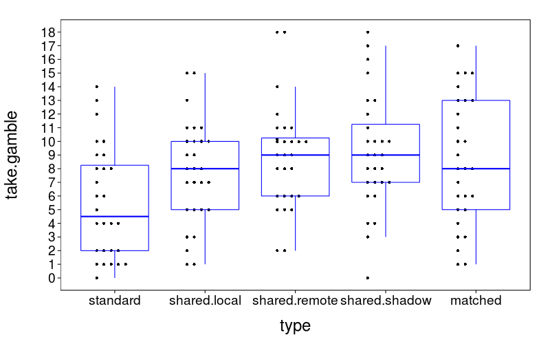
Here's a plot of the number of gambles taken for each type, collapsing across subjects.
dodge(type, take.gamble,
        data = aggregate(take.gamble ~ type + s,
            droplevels(ss(trials, type != "catch")),
            FUN = sum),
        discrete = T) +
    boxp
Now, how should modeling work? Each response is yes or no, so I'll use logistic regression. The basic per-trial predictors are:
- The subject
- The trial type
- The gamble probability
- The gamble reward
We imagine, more or less, that people are making decisions in the shared-loss trials by discounting the loss they're not exposed to by some factor representing how much they care about the victim. This suggests we should model each gamble as consisting of the components (win outcome, probability, loss outcome), where the win outcome and the probability are as specified to the subject and the loss outcome is as specified for standard and matched trials, but reduced by an unknown per-subject and per-gamble-type factor for shared-loss trials. So suppose we use these predictors per trial:
- The subject
- The gamble probability
- The gamble win outcome
- The gamble loss outcome
Where the gamble loss outcome, for shared-loss trials, is (1 + α) times half the stated loss, where α is a latent variable representing the discount factor. I imagine each subject having three αs, one for each kind of shared-loss trial. Since α ∈ [0, 1], let's model the αs as coming from beta distributions, with the only predictor being the kind of shared-loss trial (we could add a per-subject predictor, but I'm guessing it wouldn't help much).
Without shared losses
Note: The analysis in this section has not been run with the latest data.
Now, generalized linear regression is arguably a shoddy way to model risky decision-making. It certainly sounds economically unsatisfactory. This could get arbitrarily more complicated, and could be a study of its own just like Builder (a study for risk preferences what Builder was for time preferences); of course, I'd really like to avoid such madness. So let's check, considering only the standard and matched trials, that I can do a reasonable job of modeling choices in this study with a GLM.
Uh, so, after an embarrassingly long time, I realized that a really boneheaded model like choice ~ Bernoulli(ilogit(b_0 + b_1 * probability + b_2 * gain + b_3 * loss isn't gonna fly because the probability and outcomes are certaintly going to be considered dependently. The sane simple thing to do, I think, is multiply the outcomes by the probabilites in expected-value fashion: choice ~ Bernoulli(ilogit(b_0 + b_1 * probability * gain + b_3 * (1 - probability) * loss)).
model.noshared = list(

    bugs = sprintf("model %s}", paste(collapse = "\n", char(quote(
       {b0 ~ dnorm(0, 100^-2)
        b.g.gain ~ dnorm(0, 100^-2)
        b.g.loss ~ dnorm(0, 100^-2)

        b.s.sigma ~ dunif(.1, 100)
        for (s in 1 : N.subjects)
           {b.s[s] ~ dnorm(0, b.s.sigma^-2)}

        for (s in 1 : N.subjects)
           {for (g in 1 : N.gnames)
               {take.mu[g, s] <- min(1 - 1e-12, max(1e-50, ilogit(
                    b0 + b.s[s] +
                    b.g.gain * g.prob[g] * g.gain[g] +
                    b.g.loss * (1 - g.prob[g]) * g.loss[g])))
                take[g, s] ~ dbern(take.mu[g, s])
                take.pred[g, s] ~ dbern(take.mu[g, s])}}})))),

    mk.inits = function(dat) list(
        b0 = runif(1, -2, 2),
        b.g.gain = runif(1, -2, 2),
        b.g.loss = runif(1, -2, 2),
        b.s.sigma = runif(1, .1, 5)),

    jags.sample.monitor = c("take.pred"))

model.noshared.fake.p = list(
    b0 = -.5,
    b.g.gain = .07,
    b.g.loss = -.1,
    b.s.sigma = .2)

model.noshared.fake = function(trials) with(model.noshared.fake.p,
   {N.subjects = 50
    b.s = rnorm(N.subjects, 0, b.s.sigma)
    trials = ss(trials, s == levels(s)[1])
    trials = do.call(rbind, lapply(1 : N.subjects, function(sn)
        transform(
            transform(trials, s = sn, p =
                ilogit(b0 + b.s[sn] +
                    b.g.gain * gamble.prob * gamble.reward +
                    b.g.loss * (1 - gamble.prob) * gamble.reward /
                        ifelse(type == "matched", 2, 1))),
            take.gamble = rbinom(nrow(trials), 1, p))))
    transform(trials, s = factor(s))})
With fake data:
j.noshared.fake = cached(gamblejags(model.noshared,
    model.noshared.fake(ss(trials, type %in% qw(standard, matched))),
    n.chains = 4, n.adapt = 500, n.sample = 500))
gelman.diag(j.noshared.fake$samp)
| Upper C.I. | |
|---|---|
b.g.gain |
1.03 |
b.g.loss |
1.01 |
b.s.sigma |
1.07 |
b0 |
1.04 |
coda.qmean(j.noshared.fake$samp, model.noshared.fake.p)
| b.g.gain | b.g.loss | b.s.sigma | b0 | |
|---|---|---|---|---|
| hi | 0.0848 | -0.092 | 0.302 | -0.308 |
| mean | 0.0744 | -0.110 | 0.167 | -0.571 |
| true | 0.0700 | -0.100 | 0.200 | -0.500 |
| lo | 0.0636 | -0.127 | 0.102 | -0.847 |
Looks good! Now for the real data.
j.noshared.real = cached(gamblejags(model.noshared,
    ss(trials, type %in% qw(standard, matched)),
    n.chains = 5, n.adapt = 2000, thin = 2))
j.noshared.real$gnames = dimnames(j.noshared.real$data$take)[[1]]
j.noshared.real$pred = t(apply(j.noshared.real$jsamp$take.pred, c(1, 3), sum))
dimnames(j.noshared.real$pred) = list(NULL, j.noshared.real$gnames)
gelman.diag(j.noshared.real$samp)
| Upper C.I. | |
|---|---|
b.g.gain |
1.01 |
b.g.loss |
1.01 |
b.s.sigma |
1.01 |
b0 |
1.05 |
coda.qmean(j.noshared.real$samp)
| b.g.gain | b.g.loss | b.s.sigma | b0 | |
|---|---|---|---|---|
| lo | 0.112 | -0.216 | 1.20 | -4.10 |
| mean | 0.141 | -0.168 | 1.92 | -2.79 |
| hi | 0.171 | -0.124 | 3.17 | -1.45 |
This looks reasonable. b.g.gain and b.g.loss have the right signs, as does b0, since people should prefer a sure gain of $15 to a gamble for nothing. b.g.loss is greater in magnitude than b.g.gain, indicating loss aversion. b.s.sigma is appropriately large.
Now for a plot of predicted number of subjects taking each gamble. The observed number of subjects is indicated by the red dots.
with(j.noshared.real,
    coda.check(pred, sort(gnames),
        maprows(data$take, sum)[order(gnames)]) +
    theme(axis.text.x =
        element_text(size = 9, angle = 90, hjust = 1)))
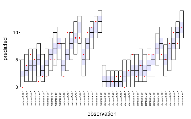
This is acceptable. In the few cases where the true value isn't in the 95% posterior interval, it isn't far. The intervals have stepladder patterns that are both empirically and theoretically appropriate. I judge this model of risky choice satisfactory for our purposes.
Individual discount factors
Let's add to the previous model the discount factors I discussed earlier.
model.idisc = list(

    bugs = sprintf("model %s}", paste(collapse = "\n", char(bquote(
       {b0 ~ dnorm(0, 100^-2)
        b.g.gain ~ dnorm(0, 100^-2)
        b.g.loss ~ dnorm(0, 100^-2)

        b.s.sigma ~ dunif(.1, 100)
        care.local.mu ~ dunif(0, 1)
        care.remote.mu ~ dunif(0, 1)
        care.shadow.mu ~ dunif(0, 1)
        care.nu ~ dunif(2, 50)
        for (s in 1 : N.subjects)
           {b.s[s] ~ dnorm(0, b.s.sigma^-2)
            care.local[s] ~ .(dbeta.munu(care.local.mu, care.nu))
            care.remote[s] ~ .(dbeta.munu(care.remote.mu, care.nu))
            care.shadow[s] ~ .(dbeta.munu(care.shadow.mu, care.nu))}

        for (s in 1 : N.subjects)
           {for (g in 1 : N.gnames)
               {take.mu[g, s] <- min(1 - 1e-12, max(1e-50, ilogit(
                    b0 + b.s[s] +
                    b.g.gain * g.prob[g] * g.gain[g] +
                    b.g.loss * (1 - g.prob[g]) *
                        (1 + ifelse(g.shared.local[g], care.local[s],
                            ifelse(g.shared.remote[g], care.remote[s],
                            ifelse(g.shared.shadow[g], care.shadow[s],
                            1)))) *
                        g.loss[g]/2)))
                take[g, s] ~ dbern(take.mu[g, s])
                take.pred[g, s] ~ dbern(take.mu[g, s])}}})))),

    mk.inits = function(dat) list(
        b0 = runif(1, -2, 2),
        b.g.gain = runif(1, -2, 2),
        b.g.loss = runif(1, -2, 2),
        b.s.sigma = runif(1, .1, 5),
        care.local.mu = runif(1, 0, 1),
        care.remote.mu = runif(1, 0, 1),
        care.shadow.mu = runif(1, 0, 1),
        care.nu = runif(1, 2, 50)),

    jags.sample.monitor = c("care.local", "care.remote", "care.shadow"))

model.idisc.fake.p = list(
    b0 = -.5,
    b.g.gain = .07,
    b.g.loss = -.1,
    b.s.sigma = .2,
    care.local.mu = .4,
    care.remote.mu = .05,
    care.shadow.mu = .2,
    care.nu = 5)

model.idisc.fake = function(trials) with(model.idisc.fake.p,
   {N.subjects = 20
    b.s = rnorm(N.subjects, 0, b.s.sigma)
    care.local = rbeta.munu(N.subjects, care.local.mu, care.nu)
    care.remote = rbeta.munu(N.subjects, care.remote.mu, care.nu)
    care.shadow = rbeta.munu(N.subjects, care.shadow.mu, care.nu)
    trials = ss(trials, s == levels(s)[1])
    trials = do.call(rbind, lapply(1 : N.subjects, function(sn)
        transform(
            transform(trials, s = sn, p =
                ilogit(b0 + b.s[sn] +
                    b.g.gain * gamble.prob * gamble.reward +
                    b.g.loss * (1 - gamble.prob) *
                        (1 + ifelse(type == "shared.local", care.local[sn],
                             ifelse(type == "shared.remote", care.remote[sn],
                             ifelse(type == "shared.shadow", care.shadow[sn],
                             ifelse(type == "matched",       0,
                             1))))) *
                        gamble.reward / 2)),
            take.gamble = rbinom(nrow(trials), 1, p))))
    transform(trials, s = factor(s))})
With fake data:
j.idisc.fake = cached(gamblejags(model.idisc,
    model.idisc.fake(trials),
    n.chains = 3, n.adapt = 1000, n.sample = 500, thin = 2))
gelman.diag(j.idisc.fake$samp)
| Upper C.I. | |
|---|---|
b.g.gain |
1.12 |
b.g.loss |
1.22 |
b.s.sigma |
1.02 |
b0 |
1.22 |
care.local.mu |
1.73 |
care.nu |
1.12 |
care.remote.mu |
2.12 |
care.shadow.mu |
2.22 |
floor(sapply(j.idisc.fake$samp, function(x) mean(x[,"care.nu"])))
| value | |
|---|---|
| 25 27 31 |
But I'm having a heck of a time getting this to fit. (Look how far off those care.nus are.) And the more I experiment with beta distributions, the less I feel they're suited for these "care" parameters. Thing is, for a given type of discount target, I expect the care parameter to be on the low side, but some substantial minority of subjects could have their care parameter near 1. That is, most subjects won't care much about the target's welfare (to a degree depending on the target), but some (and not just 1 out of 1000; more like 1 out of 8) will care about the target's welfare nearly as much as they care about their own. This suggests a mixture distribution. A rough and simple way to get this state of affairs is to have two parameters for each discount target, one which dictates the probability of a subject ever discounting, and another which dictates how much a subject discounts if they discount at all. The per-subject parameters pertaining to discounting, then, are just three dichotomous variables saying whether the subject in question discounts for the target in question.
The one thing I don't like about this new arrangement is that the handling of shadow trials is questionable. In particular, mayn't there be some subjects who refuse shadow gambles just because of the deception involved in them? Oh well, one step at a time.
Global discount factors
As a first step towards the above, let's assume all subjects discount.
Another change: I've put a stronger prior on b0. I had fitting issues where b0 got ridiculously large at least once; I can surely feel certain a priori that b0 isn't that big.
Since I had success with this model, I've moved this analysis to the second round of analyses below.
Below is the model with individual discount parameters (which didn't work out too well).
Global discount factors, individual discount flags
model.flag = list(

    bugs = sprintf("model %s}", paste(collapse = "\n", char(quote(
       {b0 ~ dunif(-4, 4)
        b.g.gain ~ dnorm(0, 100^-2)
        b.g.loss ~ dnorm(0, 100^-2)
        care.local ~ dunif(0, 1)
        care.remote ~ dunif(0, 1)
        care.shadow ~ dunif(0, 1)

        b.s.sigma ~ dunif(.1, 100)
        s.dflag.local.mu ~ dunif(0, 1)
        s.dflag.remote.mu ~ dunif(0, 1)
        s.dflag.shadow.mu ~ dunif(0, 1)
        for (s in 1 : N.subjects)
           {b.s[s] ~ dnorm(0, b.s.sigma^-2)
            s.dflag.local[s] ~ dbern(s.dflag.local.mu)
            s.dflag.remote[s] ~ dbern(s.dflag.remote.mu)
            s.dflag.shadow[s] ~ dbern(s.dflag.shadow.mu)}

        for (s in 1 : N.subjects)
           {for (g in 1 : N.gnames)
               {take.mu[g, s] <- min(1 - 1e-12, max(1e-50, ilogit(
                    b0 + b.s[s] +
                    b.g.gain * g.prob[g] * g.gain[g] +
                    b.g.loss * (1 - g.prob[g]) *
                        (1 + ifelse(g.shared.local[g],
                                ifelse(s.dflag.local[s], care.local, 1),
                            ifelse(g.shared.remote[g],
                                ifelse(s.dflag.remote[s], care.remote, 1),
                            ifelse(g.shared.shadow[g],
                                ifelse(s.dflag.shadow[s], care.shadow, 1),
                            1)))) *
                        g.loss[g]/2)))
                take[g, s] ~ dbern(take.mu[g, s])
                take.pred[g, s] ~ dbern(take.mu[g, s])}}})))),

    mk.inits = function(dat) list(
        b0 = runif(1, -2, 2),
        b.g.gain = runif(1, -2, 2),
        b.g.loss = runif(1, -2, 2),
        b.s.sigma = runif(1, .1, 5),
        s.dflag.local.mu = runif(1, 0, 1),
        s.dflag.remote.mu = runif(1, 0, 1),
        s.dflag.shadow.mu = runif(1, 0, 1),
        care.local = runif(1, 0, 1),
        care.remote = runif(1, 0, 1),
        care.shadow = runif(1, 0, 1)),

    jags.sample.monitor = c("take.pred", "s.dflag.local", "s.dflag.remote", "s.dflag.shadow"))

model.flag.fake.p = list(
    N.subjects = 50,
    b0 = -.5,
    b.g.gain = .07,
    b.g.loss = -.1,
    b.s.sigma = .2,
    s.dflag.local.mu = .7,
    s.dflag.remote.mu = .9,
    s.dflag.shadow.mu = .9,
    s.dflag.local = c(0, 1, 1, 1, 1, 0, 1, 1, 1, 0, 1, 1, 1, 1, 0, 0, 1, 1, 1, 1,  1, 1, 1, 1, 1, 1, 1, 0, 0, 0, 1, 1, 1, 1, 1, 0, 1, 0, 1, 1, 0,  1, 1, 1, 0, 1, 1, 0, 0, 1),
    s.dflag.remote = c(1, 1, 1, 1, 1, 1, 1, 1, 1, 1, 1, 1, 1, 0, 1, 1, 1, 1, 1, 1,  0, 1, 1, 1, 1, 1, 1, 1, 1, 1, 1, 1, 0, 1, 0, 1, 1, 0, 1, 1, 1,  1, 1, 1, 1, 1, 1, 0, 1, 1),
    s.dflag.shadow = c(1, 1, 1, 1, 1, 1, 1, 1, 1, 0, 1, 1, 1, 1, 1, 1, 1, 1, 1, 1,  1, 1, 1, 1, 1, 1, 0, 1, 1, 1, 1, 1, 1, 1, 1, 0, 1, 1, 0, 1, 1,  1, 1, 1, 1, 1, 1, 1, 1, 1),
    care.local = .4,
    care.remote = .05,
    care.shadow = .2)

model.flag.fake = function(trials) with(model.flag.fake.p,
   {b.s = rnorm(N.subjects, 0, b.s.sigma)
    #s.dflag.local = rbinom(N.subjects, 1, s.dflag.local.mu)
    #s.dflag.remote = rbinom(N.subjects, 1, s.dflag.remote.mu)
    #s.dflag.shadow = rbinom(N.subjects, 1, s.dflag.shadow.mu)
    trials = ss(trials, s == levels(s)[1])
    trials = do.call(rbind, lapply(1 : N.subjects, function(sn)
        transform(
            transform(trials, s = sn, p =
                ilogit(b0 + b.s[sn] +
                    b.g.gain * gamble.prob * gamble.reward +
                    b.g.loss * (1 - gamble.prob) *
                        (1 + ifelse(type == "shared.local", ifelse(s.dflag.local[sn], care.local, 1),
                             ifelse(type == "shared.remote", ifelse(s.dflag.remote[sn], care.remote, 1),
                             ifelse(type == "shared.shadow", ifelse(s.dflag.shadow[sn], care.shadow, 1),
                             ifelse(type == "matched",       0,
                             1))))) *
                        gamble.reward / 2)),
            take.gamble = rbinom(nrow(trials), 1, p))))
    transform(trials, s = factor(s))})
With fake data:
j.flag.fake = cached(gamblejags(model.flag,
    model.flag.fake(trials),
    n.chains = 4, n.adapt = 1000, n.sample = 500, thin = 2))
gelman.diag(j.flag.fake$samp)
| Upper C.I. | |
|---|---|
b.g.gain |
1.13 |
b.g.loss |
1.05 |
b.s.sigma |
1.01 |
b0 |
1.09 |
care.local |
1.00 |
care.remote |
1.02 |
care.shadow |
1.04 |
s.dflag.local.mu |
1.05 |
s.dflag.remote.mu |
1.05 |
s.dflag.shadow.mu |
1.05 |
coda.qmean(j.flag.fake$samp, model.flag.fake.p)
| b.g.gain | b.g.loss | b.s.sigma | b0 | care.local | care.remote | care.shadow | s.dflag.local.mu | s.dflag.remote.mu | s.dflag.shadow.mu | |
|---|---|---|---|---|---|---|---|---|---|---|
| hi | 0.0699 | -0.0827 | 0.284 | -0.137 | 0.8790 | 0.3740 | 0.4590 | 0.964 | 0.980 | 0.995 |
| mean | 0.0628 | -0.0946 | 0.195 | -0.318 | 0.4660 | 0.1490 | 0.2140 | 0.522 | 0.791 | 0.829 |
| true | 0.0700 | -0.1000 | 0.200 | -0.500 | 0.4000 | 0.0500 | 0.2000 | 0.700 | 0.900 | 0.900 |
| lo | 0.0558 | -0.1070 | 0.117 | -0.507 | 0.0649 | 0.0058 | 0.0205 | 0.122 | 0.524 | 0.574 |
These appear halfway reasonable. But…
transform(pred = round(pred, 3), do.call(rbind,
    lapply(qw(s.dflag.local, s.dflag.remote, s.dflag.shadow), function(p)
        cbind(p, aggregate(pred ~ true, FUN = mean, data.frame(
            true = model.flag.fake.p[[p]],
            pred = rowMeans(j.flag.fake$jsamp[[p]])))))))
| p | true | pred | |
|---|---|---|---|
| 1 | s.dflag.local | 0 | 0.654 |
| 2 | s.dflag.local | 1 | 0.579 |
| 3 | s.dflag.remote | 0 | 0.780 |
| 4 | s.dflag.remote | 1 | 0.810 |
| 5 | s.dflag.shadow | 0 | 0.808 |
| 6 | s.dflag.shadow | 1 | 0.848 |
…we can't really tell which subjects are discounting and which aren't. Those predicted probabilities differ little between the discounters and non-discounters (and for s.dflag.local, the difference is in the wrong direction). If this is the case for this fake data, which has a realistic sample size and parameter values that should be no more troublesome than the real ones, I have little hope for fitting this model to the real data.
Perhaps I should stick to model.gflag and just exclude subjects who appear not to be discounting the losses of others.
The manipulation check
Bayes attempt
I first thought of this simple Bayesian model:
tv1.model1 = list(

    bugs = sprintf("model %s}", paste(collapse = "\n", as.character(quote(
       {for (pt in 1 : (N.person.types - 1))
           {bpt[pt] ~ dnorm(0, 100^-2)}
        for (s in 1 : N.subjects)
           {dist[s, 1] <- 0
              # The social distance of person type 1 is fixed at 0.
            for (pt in 2 : N.person.types)
               {dist[s, pt] ~ dnorm(bpt[pt - 1], 1)}
            distranks[s, 1 : N.person.types] <- rank(dist[s, 1 : N.person.types])}})))),

    mk.inits = function(dat) list(
        bpt = rnorm(dat$N.person.types - 1, 1, 2)),
    jags.sample.monitor = list())

tv1.model1.fake = function()
   {N.subjects = 50
    dpt = c(1, 2, 4)
    t(replicate(N.subjects,
        rank(c(0, rnorm(length(dpt), dpt, 1)))))}
But it doesn't work. The error message JAGS gives is that a deterministic node (distranks) can't be observed. The essential problem is that I haven't stated the likelihood for distranks explicitly. And now that I've thought about it (looking at Koop and Poirier (1994)), making this work is probably much more trouble than it's worth. (Not to mention the complications that will ensue once I try to account for the subjects' dyadic connections.) Let's try something simpler.
Something simpler
ordf(aggregate(distrank ~ ptype, others, FUN = median), distrank)
| ptype | distrank | |
|---|---|---|
| 2 | parent | 1.0 |
| 1 | best_friend | 2.0 |
| 6 | occ_relative | 4.0 |
| 3 | friend_of_friend | 5.5 |
| 4 | childhood_friend | 6.0 |
| 7 | doctor | 6.0 |
| 11 | dead_relative | 6.5 |
| 8 | cashier | 7.0 |
| 5 | local_partner | 8.0 |
| 10 | unmet_classmate | 8.5 |
| 12 | stranger | 10.0 |
| 9 | remote_partner | 11.0 |
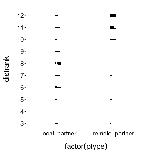
That local partner looks awfully distant, but at least they're not as distant as the remote partner.
dodge(factor(ptype), distrank,
    data = ss(others, ptype %in% qw(local_partner, remote_partner)),
    discrete = T)
Analysis: afterwards
Global discount factors model from earlier
model.gdisc = list(

    bugs = sprintf("model %s}", paste(collapse = "\n", char(quote(
       {b0 ~ dunif(-4, 4)
        b.g.gain ~ dnorm(0, 100^-2)
        b.g.loss ~ dnorm(0, 100^-2)
        care.local ~ dunif(0, 1)
        care.remote ~ dunif(0, 1)
        care.shadow ~ dunif(0, 1)

        b.s.sigma ~ dunif(.1, 100)
        for (s in 1 : N.subjects)
           {b.s[s] ~ dnorm(0, b.s.sigma^-2)}

        for (s in 1 : N.subjects)
           {for (g in 1 : N.gnames)
               {take.mu[g, s] <- min(1 - 1e-12, max(1e-50, ilogit(
                    b0 + b.s[s] +
                    b.g.gain * g.prob[g] * g.gain[g] +
                    b.g.loss * (1 - g.prob[g]) *
                        (1 + ifelse(g.shared.local[g], care.local,
                            ifelse(g.shared.remote[g], care.remote,
                            ifelse(g.shared.shadow[g], care.shadow,
                            1)))) *
                        g.loss[g]/2)))
                take[g, s] ~ dbern(take.mu[g, s])
                take.pred[g, s] ~ dbern(take.mu[g, s])}}})))),

    mk.inits = function(dat) list(
        b0 = runif(1, -2, 2),
        b.g.gain = runif(1, -2, 2),
        b.g.loss = runif(1, -2, 2),
        b.s.sigma = runif(1, .1, 5),
        care.local = runif(1, 0, 1),
        care.remote = runif(1, 0, 1),
        care.shadow = runif(1, 0, 1)),

    jags.sample.monitor = c("take.pred"))

model.gdisc.fake.p = list(
    b0 = -.5,
    b.g.gain = .07,
    b.g.loss = -.1,
    b.s.sigma = .2,
    care.local = .4,
    care.remote = .05,
    care.shadow = .2)

model.gdisc.fake = function(trials) with(model.gdisc.fake.p,
   {N.subjects = 50
    b.s = rnorm(N.subjects, 0, b.s.sigma)
    trials = ss(trials, s == levels(s)[1])
    trials = do.call(rbind, lapply(1 : N.subjects, function(sn)
        transform(
            transform(trials, s = sn, p =
                ilogit(b0 + b.s[sn] +
                    b.g.gain * gamble.prob * gamble.reward +
                    b.g.loss * (1 - gamble.prob) *
                        (1 + ifelse(type == "shared.local", care.local,
                             ifelse(type == "shared.remote", care.remote,
                             ifelse(type == "shared.shadow", care.shadow,
                             ifelse(type == "matched",       0,
                             1))))) *
                        gamble.reward / 2)),
            take.gamble = rbinom(nrow(trials), 1, p))))
    transform(trials, s = factor(s))})
With fake data:
j.gdisc.fake = cached(gamblejags(model.gdisc,
    model.gdisc.fake(trials),
    n.chains = 4, n.adapt = 1000, n.sample = 500, thin = 2))
gelman.diag(j.gdisc.fake$samp)
| Upper C.I. | |
|---|---|
b.g.gain |
1.07 |
b.g.loss |
1.02 |
b.s.sigma |
1.01 |
b0 |
1.04 |
care.local |
1.00 |
care.remote |
1.01 |
care.shadow |
1.01 |
coda.qmean(j.gdisc.fake$samp, model.gdisc.fake.p)
| b.g.gain | b.g.loss | b.s.sigma | b0 | care.local | care.remote | care.shadow | |
|---|---|---|---|---|---|---|---|
| hi | 0.0746 | -0.0848 | 0.248 | -0.235 | 0.4310 | 0.26100 | 0.483 |
| mean | 0.0672 | -0.0979 | 0.159 | -0.418 | 0.2330 | 0.09610 | 0.285 |
| true | 0.0700 | -0.1000 | 0.200 | -0.500 | 0.4000 | 0.05000 | 0.200 |
| lo | 0.0603 | -0.1100 | 0.103 | -0.590 | 0.0587 | 0.00462 | 0.103 |
Here's a table from an earlier run:
| b.g.gain | b.g.loss | b.s.sigma | b0 | care.local | care.remote | care.shadow | |
|---|---|---|---|---|---|---|---|
| hi | 0.0827 | -0.094 | 0.268 | -0.411 | 0.648 | 0.3060 | 0.30100 |
| mean | 0.0758 | -0.106 | 0.178 | -0.591 | 0.458 | 0.1300 | 0.12500 |
| true | 0.0700 | -0.100 | 0.200 | -0.500 | 0.400 | 0.0500 | 0.20000 |
| lo | 0.0691 | -0.118 | 0.105 | -0.783 | 0.285 | 0.0132 | 0.00723 |
So, I think things look okay. The error in care parameters seems to be just luck of the draw when it comes to generating the data.
Now for the real data.
j.gdisc.real = cached(gamblejags(model.gdisc,
    ss(trials, s %in% row.names(ss(sb, caught < 2))),
    n.chains = 4, n.adapt = 1000, n.sample = 2000, thin = 8))
j.gdisc.real$csamp = do.call(rbind, j.gdisc.real$samp)
j.gdisc.real$tp = j.gdisc.real$jsamp$take.pred
gelman.diag(j.gdisc.real$samp)
| Upper C.I. | |
|---|---|
b.g.gain |
1.02 |
b.g.loss |
1.01 |
b.s.sigma |
1.01 |
b0 |
1.01 |
care.local |
1.01 |
care.remote |
1.00 |
care.shadow |
1.01 |
coda.qmean(j.gdisc.real$samp)
| b.g.gain | b.g.loss | b.s.sigma | b0 | care.local | care.remote | care.shadow | |
|---|---|---|---|---|---|---|---|
| hi | 0.1170 | -0.163 | 1.250 | -1.04 | 0.437 | 0.21300 | 0.1760 |
| mean | 0.1060 | -0.188 | 0.925 | -1.52 | 0.264 | 0.08590 | 0.0646 |
| lo | 0.0954 | -0.212 | 0.680 | -1.99 | 0.107 | 0.00362 | 0.0026 |
As I said for an earlier model: "b.g.gain and b.g.loss have the right signs, as does b0, since people should prefer a sure gain of $15 to a gamble for nothing. b.g.loss is greater in magnitude than b.g.gain, indicating loss aversion." The care parameters' means are low, below .5. Very good.
c(
    "care.local > care.remote" = mean(j.gdisc.real$csamp[,"care.local"] > j.gdisc.real$csamp[,"care.remote"]),
    "care.remote > care.shadow" = mean(j.gdisc.real$csamp[,"care.remote"] > j.gdisc.real$csamp[,"care.shadow"]),
    "care.local > care.shadow" = mean(j.gdisc.real$csamp[,"care.local"] > j.gdisc.real$csamp[,"care.shadow"]))
| value | |
|---|---|
| care.local > care.remote | 0.974 |
| care.remote > care.shadow | 0.612 |
| care.local > care.shadow | 0.989 |
The care.local is very likely greater than care.remote and care.shadow. Cool.
Model checks
Let's do some posterior predictive checks to verify that this model is describing the data well. First, in analogy with fig--g/alltrials, let's look at the between-subject variability in overall number of gambles taken.
local(
   {d = data.frame(pred =
        apply(apply(j.gdisc.real$tp, c(2, 3), mean), 2, sd))
    obs = sd(colMeans(j.gdisc.real$data$take))
    ggplot(data = d) +
        geom_densitybw(aes(pred)) +
        geom_vline(x = obs, color = "red")})
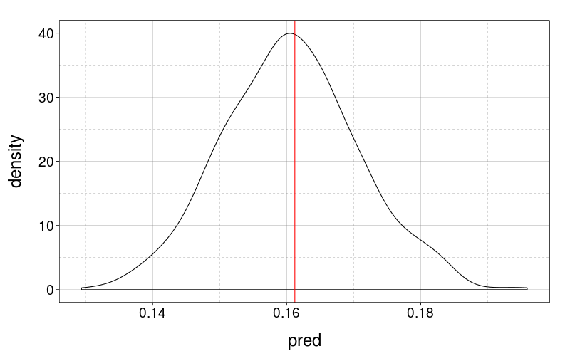
Can't ask for much better than that. I guess the model optimizes this by construction.
Now, in analogy with fig--g/count-by-type, let's examine the mean number of gambles taken per trial type.
check2 = local(
   {f = function(g)
       tapply(1 : nrow(j.gdisc.real$data$take),
           str_extract(dimnames(j.gdisc.real$data$take)[[1]], "^[^-]+"),
           g)
    list(
        obs = f(function(i)
            mean(colMeans(j.gdisc.real$data$take[i,]))),
        pred = f(function(i)
            apply(j.gdisc.real$tp[i,,], 3, mean)))})
ggplot(data = stack(check2$pred)) +
    geom_densitybw(aes(values)) +
    geom_vline(aes(xintercept = values), data = stack(check2$obs),
        color = "red") +
    facet_grid(ind ~ .) +
    theme(strip.text.y = element_text(size = 10)) + no.gridlines()
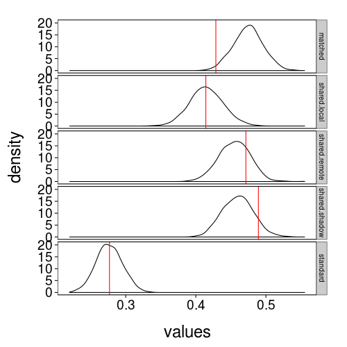
Every type looks reasonable except perhaps the matched trials. Let's look at the quantile ranks of the observed values in the predictive distributions.
with(check2, sapply(names(pred), function(type)
    ecdf(pred[[type]])(obs[type])))
| value | |
|---|---|
| matched | 0.016 |
| shared.local | 0.510 |
| shared.remote | 0.778 |
| shared.shadow | 0.917 |
| standard | 0.538 |
matched is indeed below the 2nd percentile. Looking back at fig--g/gdisc-mean-by-type, and considering how the model works, I think I see the problem, such as it is: we observed that people were a little more likely to take the remote and shadow gambles than the matched gambles, but the model allows for people to like the remote and shadow gambles at most as much as they like the matched gambles. The observation runs against the whole idea of social discounting: it suggests that people aren't discounting losses to other people so much as valuing them as small gains!
One apporach to remedying this problem is to make the model a little simpler. Right now, the effect of trial type on choice is indirect: it's fully mediated by an effect on how the loss in the given trial is treated. But suppose instead of
b0 + b.s[s] +
b.g.gain * g.prob[g] * g.gain[g] +
b.g.loss * (1 - g.prob[g]) *
    (1 + ifelse(g.shared.local[g], care.local,
        ifelse(g.shared.remote[g], care.remote,
        ifelse(g.shared.shadow[g], care.shadow,
        1)))) *
    g.loss[g]/2
we had
b0 + b.s[s] +
b.g.gain * g.prob[g] * g.gain[g] +
b.g.matched * g.matched[g] +
b.g.shared.local * g.shared.local[g] +
b.g.shared.remote * g.shared.remote[g] +
b.g.shared.shadow * g.shared.shadow[g]
One of the most substantive differences is that the latter allows matched trials to differ from standard trials in a fashion independently of how the shared trial types exert their effects.
Let's try re-expressing gdisc so that it looks more like the simpler model:
b0 + b.s[s] +
b.g.gain * g.prob[g] * g.gain[g] +
b.g.loss * (1 - g.prob[g]) * g.gain[g] * g.standard[g] +
b.g.loss * (1 - g.prob[g]) * g.gain[g]/2 * g.matched[g] +
b.g.loss * (1 - g.prob[g]) *
    (.5 + care.local/2) * g.gain[g] * g.shared.local[g] +
b.g.loss * (1 - g.prob[g]) *
    (.5 + care.remote/2) * g.gain[g] * g.shared.remote[g] +
b.g.loss * (1 - g.prob[g]) *
    (.5 + care.shadow/2) * g.gain[g] * g.shared.shadow[g]
Now another difference becomes apparent, which is that the simpler model allows the econometric characteristics of each trial to influence choice only through b.g.gain, whereas gdisc involves probability and amounts in all the trial-type terms.
And, speaking of simplicity, I'm now wondering if the "boneheaded" model I first thought of couldn't work so long as (a) an interaction term for gain and probability is added, and (b) loss amount is kept out, since its effect isn't identifiable so long as gain amount and whether-this-trial-is-a-matched-trial are kept in.
Examining umodeled factors
I've yet to use any model that accounts for subjects being in pairs. Let's see if dyad makes a difference for the kind of gamble it ought to affect the most, shared local gambles.
round(digits = 3, local(
   {v = with(ss(trials, type == "shared.local"),
       tapply(take.gamble, s, sum))
    d = t(simplify2array(tapply(row.names(sb), sb$dyad,
        function(sns) v[sns])))
    d = rbind(d, cbind(d[,2], d[,1]))   # The "double-entry" method
    cor(d[,1], d[,2])}))
| value | |
|---|---|
| -0.37 |
That's not a big correlation. Perhaps dyad can be safely ignored. How about distance ratings of the local partner?
round(digits = 3, local(
   {local.takes = with(ss(trials, type == "shared.local"),
       tapply(take.gamble, s, sum))
    dist = df2nv(ss(others, ptype == "local_partner")[qw(s, distrank)])
    cor(dist, local.takes[names(dist)], method = "spearman")}))
| value | |
|---|---|
| 0.388 |
Nor that, but notice that in this case, there's a direction to expect, and this is the right direction.
A more orthogonal model
This model more closely resembles plain logistic regression.
I've extended the prior range for b0 since its posterior seemed to be bumping up against -4.
model.orth = list(

    bugs = as.bugs.model(
       {b0 ~ dunif(-10, 10)
        b.female ~ dnorm(0, 100^-2)
        b.local.female ~ dnorm(0, 100^-2)
        b.both.female ~ dnorm(0, 100^-2)
        b.local.distrank ~ dnorm(0, 100^-2)
        b.g.egain ~ dnorm(0, 100^-2)
        b.g.matched ~ dnorm(0, 100^-2)
        b.g.shared.local ~ dnorm(0, 100^-2)
        b.g.shared.remote ~ dnorm(0, 100^-2)
        b.g.shared.shadow ~ dnorm(0, 100^-2)

        b.s.sigma ~ dunif(.1, 100)
        for (s in 1 : N.subjects)
           {b.s[s] ~ dnorm(0, b.s.sigma^-2)}

        for (s in 1 : N.subjects)
           {for (g in 1 : N.gnames)
               {take.mu[g, s] <- min(1 - 1e-12, max(1e-50, ilogit(
                    b0 +
                    b.s[s] +
                    b.female * female[s] +
                    b.local.female * local.female[s] +
                    b.both.female * female[s] * local.female[s] +
                    b.local.distrank * local.distrank[s] +
                    b.g.egain * g.prob[g] * g.gain[g] +
                    b.g.matched * g.matched[g] +
                    b.g.shared.local * g.shared.local[g] +
                    b.g.shared.remote * g.shared.remote[g] +
                    b.g.shared.shadow * g.shared.shadow[g])))
                take[g, s] ~ dbern(take.mu[g, s])
                take.pred[g, s] ~ dbern(take.mu[g, s])}}}),

    mk.inits = function(dat) list(
        b0 = runif(1, -5, 5),
        b.female = runif(1, -2, 2),
        b.local.female = runif(1, -2, 2),
        b.both.female = runif(1, -2, 2),
        b.local.distrank = runif(1, -2, 2),
        b.g.egain = runif(1, -2, 2),
        b.g.matched = runif(1, -2, 2),
        b.g.shared.local = runif(1, -2, 2),
        b.g.shared.remote = runif(1, -2, 2),
        b.g.shared.shadow = runif(1, -2, 2),
        b.s.sigma = runif(1, .1, 5)),

    jags.sample.monitor = c("take.pred"))

model.orth.fake.p = list(
    b0 = -1.5,
    b.female = -.1,
    b.local.female = .1,
    b.both.female = -.05,
    b.local.distrank = .12,
    b.g.egain = .07,
    b.g.matched = .6,
    b.g.shared.local = .2,
    b.g.shared.remote = .5,
    b.g.shared.shadow = .35,
    b.s.sigma = .2)

model.orth.fake = function(sb, trials) with(model.orth.fake.p,
   {N.subjects = 30
    sb = head(sb, N.subjects)
    row.names(sb) = c()
    b.s = rnorm(N.subjects, 0, b.s.sigma)
    trials = ss(trials, s == levels(s)[1] & type != "catch")
    trials = do.call(rbind, lapply(1 : N.subjects, function(sn)
       {female = sb[sn, "gender"] == "Female"
        local.female = sb[sn, "local.gender"] == "Female"
        transform(
            transform(trials,
                s = sn,
                p = ilogit(
                    b0 +
                    b.s[s] +
                    b.female * female +
                    b.local.female * local.female +
                    b.both.female * female * local.female +
                    b.local.distrank * sb[sn, "local.distrank"] +
                    b.g.egain * gamble.prob * gamble.reward +
                    b.g.matched * (type == "matched") +
                    b.g.shared.local * (type == "shared.local") +
                    b.g.shared.remote * (type == "shared.remote") +
                    b.g.shared.shadow * (type == "shared.shadow"))),
            take.gamble = rbinom(nrow(trials), 1, p))}))
    list(
        sb = sb[qw(gender, local.gender, local.distrank)],
        trials = transform(trials, s = factor(s)))})
With fake data:
j.orth.fake = cached(with(model.orth.fake(sb, trials), gamblejags(
    model.orth, sb, trials,
    n.chains = 4, n.adapt = 1000, n.sample = 500, thin = 2)))
j.orth.fake$csamp = do.call(rbind, j.orth.fake$samp)
gelman.diag(j.orth.fake$samp)
| Upper C.I. | |
|---|---|
b.both.female |
1.04 |
b.female |
1.04 |
b.g.egain |
1.04 |
b.g.matched |
1.02 |
b.g.shared.local |
1.00 |
b.g.shared.remote |
1.00 |
b.g.shared.shadow |
1.02 |
b.local.distrank |
1.40 |
b.local.female |
1.17 |
b.s.sigma |
1.01 |
b0 |
1.44 |
coda.qmean(j.orth.fake$samp, model.orth.fake.p)
| b.both.female | b.female | b.g.egain | b.g.matched | b.g.shared.local | b.g.shared.remote | b.g.shared.shadow | b.local.distrank | b.local.female | b.s.sigma | b0 | |
|---|---|---|---|---|---|---|---|---|---|---|---|
| hi | 0.231 | 0.4180 | 0.0776 | 0.920 | 0.439 | 0.935 | 0.6000 | 0.1820 | 0.3310 | 0.317 | -0.845 |
| mean | -0.194 | 0.0603 | 0.0673 | 0.614 | 0.140 | 0.632 | 0.2990 | 0.1160 | -0.0293 | 0.188 | -1.390 |
| true | -0.050 | -0.1000 | 0.0700 | 0.600 | 0.200 | 0.500 | 0.3500 | 0.1200 | 0.1000 | 0.200 | -1.500 |
| lo | -0.645 | -0.2750 | 0.0562 | 0.329 | -0.137 | 0.356 | 0.0396 | 0.0511 | -0.3870 | 0.106 | -2.090 |
This looks halfway reasonable. We can't say much about the gender effects, but whether that will also be the case for the real data will depend largely on the real effect size, and at any rate, they're not killing our ability to estimate the effects of actual interest.
Now for the real data.
j.orth.real = cached(gamblejags(model.orth,
    ss(sb, caught < 2), trials,
    n.chains = 8, n.adapt = 1000, n.sample = 3000, thin = 15))
j.orth.real$csamp = do.call(rbind, j.orth.real$samp)
gelman.diag(j.orth.real$samp)
| Upper C.I. | |
|---|---|
b.both.female |
1.04 |
b.female |
1.04 |
b.g.egain |
1.01 |
b.g.matched |
1.01 |
b.g.shared.local |
1.02 |
b.g.shared.remote |
1.02 |
b.g.shared.shadow |
1.02 |
b.local.distrank |
1.37 |
b.local.female |
1.12 |
b.s.sigma |
1.07 |
b0 |
1.33 |
coda.qmean(j.orth.real$samp)
| b.both.female | b.female | b.g.egain | b.g.matched | b.g.shared.local | b.g.shared.remote | b.g.shared.shadow | b.local.distrank | b.local.female | b.s.sigma | b0 | |
|---|---|---|---|---|---|---|---|---|---|---|---|
| hi | 2.020 | -0.162 | 0.0852 | 1.140 | 1.060 | 1.350 | 1.440 | 0.5970 | 1.080 | 2.110 | 2.37 |
| mean | 0.767 | -1.140 | 0.0760 | 0.846 | 0.772 | 1.060 | 1.160 | 0.0923 | -0.143 | 0.894 | -3.41 |
| lo | -0.958 | -2.370 | 0.0671 | 0.552 | 0.486 | 0.772 | 0.862 | -0.6060 | -1.420 | 0.577 | -7.87 |
round(digits = 2, prop.ranks(greater = T, cbind(zero = 0, j.orth.real$csamp[,qw(
    b0,
    b.female, b.local.female, b.both.female,
    b.g.matched, b.g.shared.local, b.g.shared.remote, b.g.shared.shadow)])))
| b.g.shared.remote | b.g.matched | b.g.shared.local | b.both.female | zero | b.local.female | b.female | b0 | |
|---|---|---|---|---|---|---|---|---|
| b.g.shared.shadow | 0.75 | 0.99 | 1.00 | 0.71 | 1.00 | 0.97 | 1.00 | 0.96 |
| b.g.shared.remote | 0.94 | 0.98 | 0.64 | 1.00 | 0.97 | 1.00 | 0.96 | |
| b.g.matched | 0.71 | 0.50 | 1.00 | 0.95 | 1.00 | 0.96 | ||
| b.g.shared.local | 0.46 | 1.00 | 0.94 | 1.00 | 0.96 | |||
| b.both.female | 0.88 | 0.80 | 0.96 | 0.96 | ||||
| zero | 0.62 | 0.99 | 0.96 | |||||
| b.local.female | 0.96 | 0.94 | ||||||
| b.female | 0.93 |
Stan
I switched to Stan because of convergence issues (notice the somewhat high PSRFs in the gelman.diag table above). This model is very similar to model.orth except that all fixed effects now have improper uniform priors.
model.sorth = list(
    stan = '
        data
           {int<lower = 0> N_subjects;
            int<lower = 0, upper = 1> female[N_subjects];
            int<lower = 0, upper = 1> local_female[N_subjects];
            int<lower = 1> local_distrank[N_subjects];
            int<lower = 0> N_gnames;
            int<lower = 0, upper = 1> take[N_gnames, N_subjects];
            real<lower = 0, upper = 1> g_prob[N_gnames];
            real<lower = 0> g_gain[N_gnames];
            int<lower = 0, upper = 1> g_matched[N_gnames];
            int<lower = 0, upper = 1> g_shared_local[N_gnames];
            int<lower = 0, upper = 1> g_shared_remote[N_gnames];
            int<lower = 0, upper = 1> g_shared_shadow[N_gnames];}
       parameters
           {real b0;
            real b_female;
            real b_local_female;
            real b_both_female;
            real b_local_distrank;
            real b_g_egain;
            real b_g_matched;
            real b_g_shared_local;
            real b_g_shared_remote;
            real b_g_shared_shadow;
            real<lower = .1, upper = 100> b_s_sigma;
            vector[N_subjects] b_s;}
        model
           {b_s ~ normal(0, b_s_sigma);
            for (s in 1 : N_subjects)
               {for (g in 1 : N_gnames)
                   {take[g, s] ~ bernoulli_logit(
                        b0 +
                        b_s[s] +
                        b_female * female[s] +
                        b_local_female * local_female[s] +
                        b_both_female * female[s] * local_female[s] +
                        b_local_distrank * local_distrank[s] +
                        b_g_egain * g_prob[g] * g_gain[g] +
                        b_g_matched * g_matched[g] +
                        b_g_shared_local * g_shared_local[g] +
                        b_g_shared_remote * g_shared_remote[g] +
                        b_g_shared_shadow * g_shared_shadow[g]);}}}',

    monitor = qw(b0, b_female, b_local_female, b_both_female, b_local_distrank, b_g_egain, b_g_matched, b_g_shared_local, b_g_shared_remote, b_g_shared_shadow),

    mk.inits = function(dat)
       {iv = model.orth$mk.inits(dat)
        c(iv, list(b_s = rnorm(dat$N.subjects, 0, iv$b.s.sigma)))})

model.sorth.fake.p = `names<-`(model.orth.fake.p,
    gsub("\\.", "_", names(model.orth.fake.p)))
With fake data:
m.sorth.fake = cached(with(model.sorth.fake(sb, trials), gamblestan(
    model.sorth, sb, trials,
    n.chains = 4)))
round(summary(m.sorth.fake, pars = model.sorth$monitor)$summary[,"Rhat"], 3)
| value | |
|---|---|
| b0 | 1.003 |
| b_female | 1.002 |
| b_local_female | 1.000 |
| b_both_female | 1.002 |
| b_local_distrank | 1.002 |
| b_g_egain | 1.001 |
| b_g_matched | 1.002 |
| b_g_shared_local | 1.001 |
| b_g_shared_remote | 1.000 |
| b_g_shared_shadow | 1.001 |
stan.qmean(
    extract(m.sorth.fake, pars = names(model.sorth.fake.p)),
    model.sorth.fake.p)
| b0 | b_female | b_local_female | b_both_female | b_local_distrank | b_g_egain | b_g_matched | b_g_shared_local | b_g_shared_remote | b_g_shared_shadow | b_s_sigma | |
|---|---|---|---|---|---|---|---|---|---|---|---|
| hi | -0.917 | 0.231 | 0.3140 | 0.512 | 0.1920 | 0.0790 | 1.120 | 0.5290 | 0.850 | 0.5110 | 0.293 |
| mean | -1.520 | -0.126 | -0.0263 | 0.052 | 0.1360 | 0.0685 | 0.820 | 0.2500 | 0.562 | 0.2280 | 0.165 |
| true | -1.500 | -0.100 | 0.1000 | -0.050 | 0.1200 | 0.0700 | 0.600 | 0.2000 | 0.500 | 0.3500 | 0.200 |
| lo | -2.080 | -0.474 | -0.3700 | -0.422 | 0.0795 | 0.0583 | 0.502 | -0.0191 | 0.274 | -0.0575 | 0.103 |
Very good.
Now for the real data.
m.sorth.real = cached(gamblestan(model.sorth,
    ss(sb, caught < 2), trials,
    n.chains = 8, iter = 500))
round(digits = 3, summary(m.sorth.real,
    pars = c(model.sorth$monitor, "b_s_sigma"))$summary[,"Rhat"])
| value | |
|---|---|
| b0 | 1.006 |
| b_female | 1.011 |
| b_local_female | 1.029 |
| b_both_female | 1.016 |
| b_local_distrank | 1.003 |
| b_g_egain | 1.002 |
| b_g_matched | 1.000 |
| b_g_shared_local | 1.001 |
| b_g_shared_remote | 0.999 |
| b_g_shared_shadow | 1.001 |
| b_s_sigma | 1.003 |
stan.qmean(extract(m.sorth.real, pars = model.sorth$monitor))
| b0 | b_female | b_local_female | b_both_female | b_local_distrank | b_g_egain | b_g_matched | b_g_shared_local | b_g_shared_remote | b_g_shared_shadow | |
|---|---|---|---|---|---|---|---|---|---|---|
| hi | -2.32 | -0.433 | 0.606 | 2.3200 | 0.248 | 0.0876 | 1.080 | 1.020 | 1.270 | 1.380 |
| mean | -3.55 | -1.240 | -0.296 | 1.1100 | 0.100 | 0.0796 | 0.817 | 0.744 | 1.000 | 1.100 |
| lo | -4.82 | -2.110 | -1.140 | -0.0751 | -0.039 | 0.0720 | 0.533 | 0.483 | 0.748 | 0.842 |
round(digits = 3, prop.ranks(greater = T, cbind(zero = 0,
    do.call(cbind, extract(m.sorth.real, pars =
        qw(b_g_matched, b_g_shared_local, b_g_shared_remote, b_g_shared_shadow))))))
| b_g_shared_remote | b_g_matched | b_g_shared_local | zero | |
|---|---|---|---|---|
| b_g_shared_shadow | 0.781 | 0.991 | 0.998 | 1.000 |
| b_g_shared_remote | 0.906 | 0.974 | 1.000 | |
| b_g_matched | 0.702 | 1.000 | ||
| b_g_shared_local | 1.000 |
- It's >99% likely that all kinds of shared gambles, as well as matched gambles, were more appealing than standard gambles.
- It's 99% likely that shadow gambles were more appealing than matched gambles.
- It's >95% that remote and shadow gambles were more appealing than local gambles.
- It's 78% likely that shadow gambles were more appealing than remote gambles.
sapply(extract(m.sorth.real, pars = qw(b_female, b_local_female)),
    function(v) mean(v < 0))
| value | |
|---|---|
| b_female | 0.9965 |
| b_local_female | 0.7610 |
mean(rowSums(simplify2array(extract(m.sorth.real, pars =
      qw(b_female, b_local_female, b_both_female))))
  < 0)
| value | |
|---|---|
| 0.868 |
rd(qmean(simplify2array(extract(m.sorth.real, pars =
    qw(b_female, b_local_female, b_both_female)))))
| value | |
|---|---|
| lo | -1.836 |
| mean | -0.144 |
| hi | 2.038 |
local(
   {m = do.call(cbind, extract(m.sorth.real, pars =
        qw(b_female, b_local_female, b_both_female)))
    m = transform(m,
        b_both_female = b_both_female + b_local_female + b_female,
        zero = 0)
    names(m) = qw(F2M, M2F, F2F, M2M)
    round(prop.ranks(greater = T, m), 3)})
| M2F | F2F | F2M | |
|---|---|---|---|
| M2M | 0.761 | 0.868 | 0.996 |
| M2F | 0.626 | 0.982 | |
| F2F | 0.958 |
The clearest finding here is just that women with male partners were least likely to take gambles.
Now, about the social-distance measure. Did it relate to choices much? At the very least, we'd expect greater social distance to be associated with more, not less, willingness to take gambles.
mean(extract(m.sorth.real, pars = "b_local_distrank")[[1]] > 0)
| value | |
|---|---|
| 0.92 |
That probability isn't as high as one might hope. Let's see how strong the effect of social distance is. First, here are the frequencies of social-distance ratings for the local partner.
table(ss(sb, caught < 2)$local.distrank)
| count | |
|---|---|
| 3 | 2 |
| 5 | 1 |
| 6 | 6 |
| 7 | 2 |
| 8 | 10 |
| 9 | 4 |
| 10 | 1 |
| 11 | 4 |
| 12 | 2 |
Let's try comparing ranks 11 and 6, since they're extreme but not too extreme.
local(
   {p = extract(m.sorth.real, pars = "b_local_distrank")[[1]]
    round(digits = 3, qmean(p * 11 - p * 6))})
| value | |
|---|---|
| lo | -0.195 |
| mean | 0.502 |
| hi | 1.242 |
A difference of .5 logits would increase a choice probability of 50% to ilogit(.5) = 62%. That's something, but it isn't large. By comparison, the posterior mean of b_shared_remote is 1, which would increase 50% to 73%. But the posterior interval for b_local_distrank is wide, so the effect of social distance might credibly be much stronger.
With all subjects
Let's check how the analyses presented in the paper change when the two excluded subjects are put back in.
round(d = 2, with(trials, tapply(take.gamble, type, mean)))
| value | |
|---|---|
| catch | 0.08 |
| standard | 0.30 |
| shared.local | 0.41 |
| shared.remote | 0.45 |
| shared.shadow | 0.47 |
| matched | 0.43 |
Very similar (no big surprise; these are just proportions).
m.sorth.all = cached(gamblestan(model.sorth,
    sb, trials,
    n.chains = 8, iter = 500))
round(digits = 3, summary(m.sorth.all,
    pars = c(model.sorth$monitor, "b_s_sigma"))$summary[,"Rhat"])
| value | |
|---|---|
| b0 | 1.012 |
| b_female | 1.020 |
| b_local_female | 1.018 |
| b_both_female | 1.013 |
| b_local_distrank | 1.010 |
| b_g_egain | 1.000 |
| b_g_matched | 1.010 |
| b_g_shared_local | 1.006 |
| b_g_shared_remote | 1.007 |
| b_g_shared_shadow | 1.005 |
| b_s_sigma | 1.000 |
d = melt(extract(m.sorth.all, perm = T, pars =
    qw(b_g_matched, b_g_shared_local, b_g_shared_remote, b_g_shared_shadow)))
d$L1 = factor(d$L1)
levels(d$L1) = sub("shadow", "deceit", sub("^b_g_", "", levels(d$L1)))
ggplot(d) +
    stat_summary(aes(L1, value), fun.data = function(y)
        data.frame(y = mean(y), ymin = quantile(y, .025), ymax = quantile(y, .975))) +
    coord_cartesian(ylim = c(.4, 1.4)) +
    xlab("Parameter (b_g_…)") + ylab("Value") +
    no.gridlines()
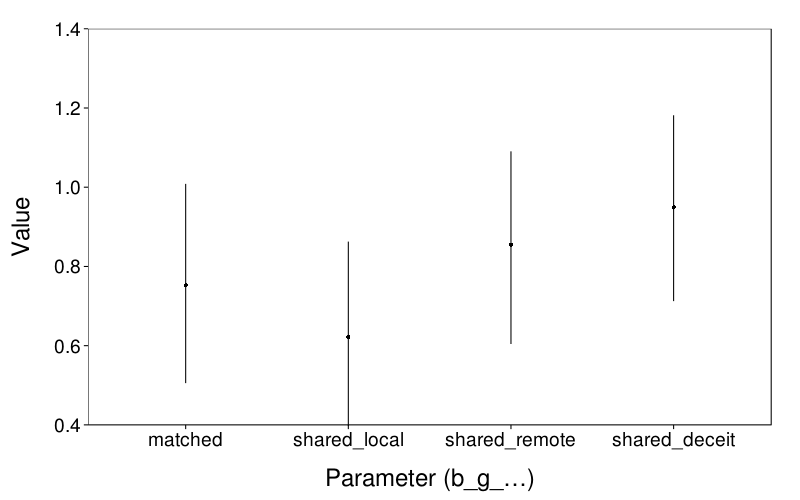
All these parameters shrank, but their relative sizes look similar.
tab = prop.ranks(greater = T, cbind(zero = 0,
    do.call(cbind, extract(m.sorth.all, pars =
        qw(b_g_matched, b_g_shared_local, b_g_shared_remote, b_g_shared_shadow)))))
tab = ss(melt(tab), !is.na(value))
for (col in 1:2)
    tab[,col] = gsub("shadow", "deceit", gsub("b_g(_shared)?_", "", tab[,col]))
v = tab$value
names(v) = maprows(tab, function(v)
    paste(sort(c(v["Var1"], v["Var2"])), collapse = "."))
round(d = 3, as.matrix(data.frame(
    row.names =     qw(b_g_shared_deceit, b_g_shared_remote, b_g_shared_local, b_g_matched),
    b_g_shared_remote = c(v["deceit.remote"], NA,        NA,           NA),
    b_g_shared_local =  c(v["deceit.local"], v["local.remote"], NA,      NA),
    b_g_matched =       c(v["deceit.matched"], v["matched.remote"], 1 - v["local.matched"], NA),
    zero =          v[qw(deceit.zero, remote.zero, local.zero, matched.zero)])))
| b_g_shared_remote | b_g_shared_local | b_g_matched | zero | |
|---|---|---|---|---|
| b_g_shared_deceit | 0.778 | 0.998 | 0.952 | 1.000 |
| b_g_shared_remote | 0.974 | 0.800 | 1.000 | |
| b_g_shared_local | 0.135 | 1.000 | ||
| b_g_matched | 1.000 |
Generally, the probabilities are comparable. The biggest differences are for local versus matched (which got stronger) and remote versus matched (which got weaker, but who cares about that comparison, anyway?).
mean(extract(m.sorth.all, "b_local_distrank")[[1]] > 0)
| value | |
|---|---|
| 0.894 |
Not too different.
ANOVA
Let's do a traditional sloppy little ANOVA in case it will help reviewers accept the main analysis.
gtype.props = droplevels(aggregate(take.gamble ~ s + type,
    ss(trials, type != "catch" &
        s %in% row.names(ss(sb, caught < 2))),
    mean))
anova.gt = aov(take.gamble ~ type + Error(s / type),
    data = gtype.props)
c(p = summary(anova.gt)[[2]][[1]]["type", "Pr(>F)"])
| value | |
|---|---|
| p | 3.056963e-06 |
So the overall model is significant. For follow-up, let's use dependent-samples t-tests.
n = length(unique(gtype.props$s))
tvs = with(gtype.props,
   {c(recursive = T, lapply(levels(type), function(type1)
        lapply(setdiff(levels(type), type1), function(type2)
           {t = t.test(paired = T, var.eq = T,
                take.gamble[type == type1],
                take.gamble[type == type2])$statistic
            `names<-`(abs(t), paste(collapse = " > ",
                (if (t < 0) c(type2, type1) else c(type1, type2))))})))})
tvs = tvs[sort(unique(names(tvs)))]
round(d = 3, cbind(
    t = tvs,
    p = 2 * pt(abs(tvs), n - 1, lower = F)))
| t | p | |
|---|---|---|
| matched > shared.local | 0.270 | 0.789 |
| matched > standard | 4.576 | 0.000 |
| shared.local > standard | 3.707 | 0.001 |
| shared.remote > matched | 0.746 | 0.461 |
| shared.remote > shared.local | 1.771 | 0.086 |
| shared.remote > standard | 4.863 | 0.000 |
| shared.shadow > matched | 1.160 | 0.255 |
| shared.shadow > shared.local | 2.871 | 0.007 |
| shared.shadow > shared.remote | 0.844 | 0.405 |
| shared.shadow > standard | 4.874 | 0.000 |
All comparisons against standard gambles are significant, as is shadow versus local.
TV 4
Prescreens
tv4.s = row.names(ss(sb, tv == 4 & caught < 2))
repcond = sb[tv4.s, "repcond"]
rbind(as.matrix(data.frame(row.names = "n", Anonymous = sum(repcond == "Anonymous"), Visible = sum(repcond == "Visible"))),
    do.call(rbind, lapply(colnames(prescreens), function(v)
       {x = prescreens[tv4.s, v]
        if (is.factor(x))
            x = droplevels(x)
        d = as.data.frame.matrix(table(x, repcond, useNA = "ifany"))
        row.names(d) = paste0("    ", row.names(d))
        as.matrix(rbind(
            data.frame(row.names = v, Anonymous = NA, Visible = NA),
            d))})))
| Anonymous | Visible | |
|---|---|---|
| n | 17 | 17 |
| gender | ||
| Female | 10 | 11 |
| Male | 7 | 6 |
| age | ||
| 18 | 10 | 6 |
| 19 | 3 | 0 |
| 20 | 3 | 4 |
| 21 | 0 | 2 |
| 22 | 1 | 3 |
| 23 | 0 | 1 |
| 27 | 0 | 1 |
| race | ||
| Asian | 4 | 4 |
| Black | 1 | 1 |
| Multi | 0 | 1 |
| MultiH | 0 | 1 |
| NatAm | 1 | 0 |
| Other | 1 | 0 |
| White | 9 | 8 |
| WhiteH | 1 | 2 |
| sexo | ||
| Het | 14 | 15 |
| Gay | 1 | 0 |
| Bi | 1 | 1 |
| NA | 1 | 1 |
| year | ||
| Freshman | 11 | 6 |
| Sophomore | 2 | 0 |
| Junior | 4 | 5 |
| Senior | 0 | 4 |
| SuperSenior | 0 | 1 |
| NA | 0 | 1 |
| english | ||
| Native | 17 | 17 |
| nativelang | ||
| English | 17 | 17 |
| bilingual | ||
| No | 13 | 13 |
| Yes | 4 | 4 |
| hand | ||
| Left | 2 | 1 |
| Right | 15 | 16 |
| normalvision | ||
| No | 2 | 0 |
| Yes | 15 | 17 |
| colorblind | ||
| No | 17 | 17 |
This table is a breakdown of all questions asked in Stony Brook's subject-pool prescreen by condition in Study 1. In the table:
NAvalues are from subjects who didn't answer the corresponding question or chose a "don't know" option.MultiHandWhiteHvalues are from subjects who indicated they were Hispanic on a yes-or-no item seperate from the main race item.handasked subjects their dominant hand.normalvisionasked whether subjects had normal or corrected-to-normal visual acuity.
It looks like the samples were largely similar with the exception that the Visible group was somewhat older than the Anonymous group.
Descriptive
ses = row.names(ss(sb, tv == 4 & caught < 2))
c("Sample size" = length(ses),
    "In anonymous condition" = sum(sb[ses, "repcond"] == "Anonymous"),
    "In visible condition" = sum(sb[ses, "repcond"] == "Visible"))
| value | |
|---|---|
| Sample size | 34 |
| In anonymous condition | 17 |
| In visible condition | 17 |
ts = transform(ss(trials, char(s) %in% ses & type == "shared.local"),
    gname = factor(gname, levels = sort(levels(factor(gname)))),
    repcond = sb[char(s), "repcond"])
x = transform(dcast(aggregate(take.gamble ~ repcond + gname, ts, sum),
    gname ~ repcond, value.var = "take.gamble"),
  anon.inc = Anonymous - Visible)
x
| gname | Anonymous | Visible | anon.inc | |
|---|---|---|---|---|
| 1 | shared.local-5-20 | 7 | 3 | 4 |
| 2 | shared.local-5-30 | 7 | 6 | 1 |
| 3 | shared.local-5-40 | 8 | 11 | -3 |
| 4 | shared.local-5-50 | 7 | 11 | -4 |
| 5 | shared.local-5-60 | 9 | 8 | 1 |
| 6 | shared.local-6-20 | 1 | 5 | -4 |
| 7 | shared.local-6-30 | 4 | 7 | -3 |
| 8 | shared.local-6-40 | 13 | 10 | 3 |
| 9 | shared.local-6-50 | 10 | 8 | 2 |
| 10 | shared.local-6-60 | 12 | 13 | -1 |
| 11 | shared.local-7-20 | 5 | 5 | 0 |
| 12 | shared.local-7-30 | 19 | 10 | 9 |
| 13 | shared.local-7-40 | 17 | 10 | 7 |
| 14 | shared.local-7-50 | 23 | 16 | 7 |
| 15 | shared.local-7-60 | 22 | 20 | 2 |
| 16 | shared.local-8-20 | 18 | 8 | 10 |
| 17 | shared.local-8-30 | 22 | 18 | 4 |
| 18 | shared.local-8-40 | 22 | 19 | 3 |
| 19 | shared.local-8-50 | 24 | 24 | 0 |
| 20 | shared.local-8-60 | 26 | 24 | 2 |
Here is the number of times in each condition each shared local gamble was taken. The last column is simply Anonymous minus Visible.
For NHST:
l = t.test(x$anon.inc, mu = 0, var.eq = T)
round(d = 3, with(l, c(statistic, parameter, p = p.value)))
| value | |
|---|---|
| t | 2.20 |
| df | 19.00 |
| p | 0.04 |
Bayes
I've omitted b_both_female because it would create identifiability issues because our sample for TV 4 has no male–male pairs.
model.sorth.tv4 = list(
    stan = '
        data
           {int<lower = 0> N_subjects;
            int<lower = 0, upper = 1> female[N_subjects];
            int<lower = 0, upper = 1> local_female[N_subjects];
            int<lower = 0, upper = 1> anonymous[N_subjects];
            int<lower = 0> N_gnames;
            int<lower = 0, upper = 1> take[2, N_gnames, N_subjects];
            real<lower = 0, upper = 1> g_prob[N_gnames];
            real<lower = 0> g_gain[N_gnames];
            int<lower = 0, upper = 1> g_shared_local[N_gnames];}
       parameters
           {real b0;
            real b_female;
            real b_local_female;
            real b_g_egain;
            real b_g_shared_anon;
            real b_g_shared_visible;
            real<lower = .1, upper = 100> b_s_sigma;
            vector[N_subjects] b_s;}
        model
           {b_s ~ normal(0, b_s_sigma);
            for (s in 1 : N_subjects) {for (g in 1 : N_gnames) {for (iter in 1 : 2)
                take[iter, g, s] ~ bernoulli_logit(
                    b0 +
                    b_s[s] +
                    b_female * female[s] +
                    b_local_female * local_female[s] +
                    b_g_egain * g_prob[g] * g_gain[g] +
                    b_g_shared_anon * g_shared_local[g] * anonymous[s] +
                    b_g_shared_visible * g_shared_local[g] * !anonymous[s]);}}}',

    monitor = qw(b0, b_female, b_local_female, b_g_egain, b_g_shared_anon, b_g_shared_visible),

    mk.inits = function(dat)
       {l = list(
            b0 = runif(1, -5, 5),
            b.female = runif(1, -2, 2),
            b.local.female = runif(1, -2, 2),
            b.g.egain = runif(1, -2, 2),
            b.g.shared.anon = runif(1, -2, 2),
            b.g.shared.visible = runif(1, -2, 2),
            b.s.sigma = runif(1, .1, 5))
        l$b.s = rnorm(dat$N.subjects, 0, l$b.s.sigma)
        l})

model.sorth.tv4.fake.p = list(
    b0 = -2.5,
    b_female = -.1,
    b_local_female = .1,
    b_g_egain = .1,
    b_g_shared_anon = .4,
    b_g_shared_visible = .1,
    b_s_sigma = .2)

model.sorth.tv4.fake = function(sb, trials) with(model.sorth.tv4.fake.p,
   {N.subjects = 25

    sb = head(ss(sb, tv == 4), N.subjects)
    gendm = reprows(len = nrow(sb),
        expand.grid(gender = qw(Male, Female), local.gender = qw(Male, Female)))
    sb$female = gendm$female
    sb$local.gender = gendm$local.gender

    b_s = rnorm(N.subjects, 0, b_s_sigma)
    trials = ss(trials, s == row.names(sb)[1] & type != "catch")
    row.names(sb) = c()
    trials = do.call(rbind, lapply(1 : N.subjects, function(sn)
       {female = sb[sn, "gender"] == "Female"
        local.female = sb[sn, "local.gender"] == "Female"
        anonymous = sb[sn, "repcond"] == "Anonymous"
        transform(
            transform(trials,
                s = sn,
                p = ilogit(
                    b0 +
                    b_s[sn] +
                    b_female * female +
                    b_local_female * local.female +
                    b_g_egain * gamble.prob * gamble.reward +
                    b_g_shared_anon * (type == "shared.local") * anonymous +
                    b_g_shared_visible * (type == "shared.local") * !anonymous)),
            take.gamble = rbinom(nrow(trials), 1, p))}))
    list(
        sb = sb[qw(gender, local.gender, repcond)],
        trials = transform(trials, s = factor(s)))})
With fake data:
m.sorth.tv4.fake = cached(with(model.sorth.tv4.fake(sb, trials), gamblestan(
    model.sorth.tv4, sb, trials,
    n.chains = 4, iter = 500, refresh = 100)))
round(summary(m.sorth.tv4.fake,
    pars = c(model.sorth.tv4$monitor, "b_s_sigma"))$summary[,"Rhat"], 3)
| value | |
|---|---|
| b0 | 1.006 |
| b_female | 1.003 |
| b_local_female | 1.007 |
| b_both_female | 1.007 |
| b_g_egain | 0.998 |
| b_g_shared_anon | 1.003 |
| b_g_shared_visible | 0.998 |
| b_s_sigma | 1.004 |
stan.qmean(
    extract(m.sorth.tv4.fake, pars = names(model.sorth.tv4.fake.p)),
    model.sorth.tv4.fake.p)
| b0 | b_female | b_local_female | b_both_female | b_g_egain | b_g_shared_anon | b_g_shared_visible | b_s_sigma | |
|---|---|---|---|---|---|---|---|---|
| hi | -2.31 | 0.3650 | 0.4380 | 0.49500 | 0.1130 | 0.705 | 0.3550 | 0.303 |
| mean | -2.70 | 0.0016 | 0.0129 | -0.00397 | 0.1010 | 0.469 | 0.0838 | 0.170 |
| true | -2.50 | -0.1000 | 0.1000 | -0.05000 | 0.1000 | 0.400 | 0.1000 | 0.200 |
| lo | -3.08 | -0.3350 | -0.3770 | -0.51200 | 0.0906 | 0.239 | -0.1700 | 0.103 |
Not bad.
x = do.call(cbind, extract(m.sorth.tv4.fake, pars =
    qw(b_g_shared_anon, b_g_shared_visible)))
mean(x[,"b_g_shared_anon"] > x[,"b_g_shared_visible"])
| value | |
|---|---|
| 0.996 |
Now for the real data.
m.sorth.tv4.real = cached(gamblestan(model.sorth.tv4,
    ss(sb, tv == 4 & caught < 2), trials,
    n.chains = 8, iter = 500))
round(digits = 3, summary(m.sorth.tv4.real,
    pars = c(model.sorth.tv4$monitor, "b_s_sigma"))$summary[,"Rhat"])
| value | |
|---|---|
| b0 | 1.017 |
| b_female | 1.028 |
| b_local_female | 1.026 |
| b_g_egain | 0.998 |
| b_g_shared_anon | 1.004 |
| b_g_shared_visible | 1.000 |
| b_s_sigma | 1.008 |
stan.qmean(
    extract(m.sorth.tv4.real, pars = model.sorth.tv4$monitor))
| b0 | b_female | b_local_female | b_g_egain | b_g_shared_anon | b_g_shared_visible | |
|---|---|---|---|---|---|---|
| hi | -1.90 | 0.766 | 0.608 | 0.0925 | 0.943 | 0.185 |
| mean | -2.89 | -0.113 | -0.260 | 0.0833 | 0.682 | -0.059 |
| lo | -4.03 | -0.909 | -1.070 | 0.0743 | 0.417 | -0.304 |
x = do.call(cbind, extract(m.sorth.tv4.real, pars =
    qw(b_g_shared_anon, b_g_shared_visible)))
mean(x[,"b_g_shared_anon"] > x[,"b_g_shared_visible"])
| value | |
|---|---|
| 1 |
sapply(extract(m.sorth.tv4.real, pars = qw(b_female, b_local_female)),
    function(v) mean(v < 0))
| value | |
|---|---|
| b_female | 0.6230 |
| b_local_female | 0.7415 |
More NHST
These tests don't account for the nuisance variables in the regression models, such as win probability and gender. This arguably breaks the ordinal scale of the data.
For Study 1, comparing the rate of taking shared gambles between conditions, using a Mann–Whitney U-test per reviewer 1:
takes.shared = with(
    ss(trials,
        s %in% row.names(ss(sb, tv == 4 & caught < 2)) &
        type == "shared.local"),
    tapply(take.gamble, droplevels(s), sum))
repconds = sb[names(takes.shared), "repcond"]
w = wilcox.test(takes.shared ~ repconds,
    exact = F, # Exact p-values not available with ties.
    correct = F)
rd(c(U = unname(w$statistic), p = w$p.value))
| value | |
|---|---|
| U | 167.500 |
| p | 0.427 |
For Study 1, comparing moral-hazard scores (shared gambles taken minus standard gambles taken) between conditions:
takes.standard = with(
    ss(trials,
        s %in% row.names(ss(sb, tv == 4 & caught < 2)) &
        type == "standard"),
    tapply(take.gamble, droplevels(s), sum))[names(takes.shared)]
mh = takes.shared - takes.standard
w = wilcox.test(mh ~ repconds,
    exact = F,
    correct = F)
rd(c(U = unname(w$statistic), p = w$p.value))
| value | |
|---|---|
| U | 193.50 |
| p | 0.09 |
For Study 2, comparing the rate of gamble acceptance between gamble types, using signed-rank tests:
d = droplevels(aggregate(take.gamble ~ s + type,
    ss(trials, type != "catch" &
        s %in% row.names(ss(sb, tv <= 3 & caught < 2))),
    sum))
combs = combn(levels(d$type), 2)
s = do.call(rbind, lapply(1 : ncol(combs), function(ci)
   {type1 = combs[1, ci]
    type2 = combs[2, ci]
    t1 = d$take.gamble[d$type == type1]
    t2 = d$take.gamble[d$type == type2]
    if (mean(t1 > t2) > .5)
      # Swap.
        vassign(.(type1, type2, t1, t2), list(type2, type1, t2, t1))
    w = wilcox.test(t1, t2,
        paired = T, exact = F, correct = F)
    data.frame(
        row.names = sprintf("%s > %s", type2, type1),
        W = abs(w$statistic),
        p = w$p.value)}))
s = s[order(row.names(s)),]
s[,"Sig. (α = .05)"] = s$p <= .05
s[,sprintf("Sig. (α = %s)", substr(.05 / nrow(s), 2, 1e9))] = s$p <= .05 / nrow(s)
rd(d = 5, s)
| W | p | Sig. (α = .05) | Sig. (α = .005) | |
|---|---|---|---|---|
| matched > standard | 25.0 | 0.00002 | TRUE | TRUE |
| shared.local > matched | 221.0 | 0.93946 | FALSE | FALSE |
| shared.local > standard | 81.0 | 0.00175 | TRUE | TRUE |
| shared.remote > matched | 160.0 | 0.32580 | FALSE | FALSE |
| shared.remote > shared.local | 112.0 | 0.06252 | FALSE | FALSE |
| shared.remote > standard | 35.0 | 0.00005 | TRUE | TRUE |
| shared.shadow > matched | 163.5 | 0.15469 | FALSE | FALSE |
| shared.shadow > shared.local | 90.5 | 0.00956 | TRUE | FALSE |
| shared.shadow > shared.remote | 145.5 | 0.18380 | FALSE | FALSE |
| shared.shadow > standard | 48.0 | 0.00014 | TRUE | TRUE |
For Study 2, comparing the social-distance ranks of local and remote partners with a signed-rank test:
d = distranks[row.names(ss(sb, tv <= 3 & caught < 2)), qw(local_partner, remote_partner)]
w = wilcox.test(d$local_partner, d$remote_partner,
    paired = T, exact = F, correct = F)
rd(d = 4, c(W = unname(w$statistic), p = w$p.value))
| value | |
|---|---|
| W | 64.5000 |
| p | 0.0002 |
References
Koop, G., & Poirier, D. J. (1994). Rank-ordered logit models: An empirical analysis of Ontario voter preferences. Journal of Applied Econometrics, 9(4), 369–388. doi:10.1002/jae.3950090406