Leaf notebook
Created 3 Apr 2014 • Last modified 24 Mar 2015
Subjects
bad.s
| x | |
|---|---|
| 1 | s25 |
| 2 | s31 |
| 3 | s51 |
| 4 | s52 |
| 5 | s71 |
| 6 | s80 |
maybe.bad.s
| x | |
|---|---|
| 1 | s52 |
| 2 | s54 |
| 3 | s56 |
Choice GLMMs
choice.lreg = function(d) glmer(
    choice ~
        payoff_condition * show_opponent_score +
        opponent_choice +
        (1|subject),
    data = d,
    family = binomial(link = "logit"))

model.summary = function(model)
    {x = round(summary(model)@coefs, 3)
     colnames(x)[ncol(x)] = "p"
     x}
model.summary(choice.lreg(ss(ts,
    !(char(subject) %in% bad.s))))
| Estimate | Std. Error | z value | p | |
|---|---|---|---|---|
| (Intercept) | -4.114 | 0.337 | -12.197 | 0.000 |
| payoff_condition1-2-9-10 | -0.253 | 0.132 | -1.912 | 0.056 |
| show_opponent_scoreTrue | 1.779 | 0.444 | 4.009 | 0.000 |
| opponent_choiceCooperate | 1.358 | 0.075 | 17.984 | 0.000 |
| payoff_condition1-2-9-10:show_opponent_scoreTrue | 0.659 | 0.158 | 4.169 | 0.000 |
Here is the proportions of trials that were cooperations stratified by condition:
m = with(ss(ts, !(char(subject) %in% bad.s)),
   {f = function(v) tapply(choice == "Cooperate", v, mean)
    rbind(
        f(show_opponent_score == "True"),
        f(opponent_choice == "Cooperate"),
        f((payoff_condition == "1-2-9-10") & (show_opponent_score == "True")),
        f((payoff_condition == "1-2-9-10") & (show_opponent_score == "False")))})
dimnames(m)[[1]] = qw(show_opponent_score, opponent_cooperates, payoff_condition_129X_withscore, payoff_condition_129X_noscore)
round(d = 2, m[,c(2,1)])
| TRUE | FALSE | |
|---|---|---|
| show_opponent_score | 0.28 | 0.11 |
| opponent_cooperates | 0.28 | 0.12 |
| payoff_condition_129X_withscore | 0.32 | 0.16 |
| payoff_condition_129X_noscore | 0.10 | 0.23 |
model.summary(choice.lreg(ss(ts,
    !(char(subject) %in% union(bad.s, maybe.bad.s)))))
| Estimate | Std. Error | z value | p | |
|---|---|---|---|---|
| (Intercept) | -4.174 | 0.347 | -12.023 | 0.000 |
| payoff_condition1-2-9-10 | -0.353 | 0.137 | -2.583 | 0.010 |
| show_opponent_scoreTrue | 1.837 | 0.456 | 4.028 | 0.000 |
| opponent_choiceCooperate | 1.384 | 0.077 | 17.953 | 0.000 |
| payoff_condition1-2-9-10:show_opponent_scoreTrue | 0.714 | 0.163 | 4.387 | 0.000 |
With social distance
Here, I've calculated social distance (pdist.r) as the rank of a score from a simple within-subject linear regression. This should be robust to various scaling issues like how generous subjects are in general.
choice.lreg.pdist = function(var, d) glmer(
    choice ~
        payoff_condition +
        get(var) +
        opponent_choice +
        (1|subject),
    data = ss(d, show_opponent_score == "True"),
    family = binomial(link = "logit"))
model.summary(choice.lreg.pdist("pdist.r", ss(ts,
    !(char(subject) %in% bad.s) & !is.na(pdist.r))))
| Estimate | Std. Error | z value | p | |
|---|---|---|---|---|
| (Intercept) | -2.641 | 0.483 | -5.473 | 0.000 |
| payoff_condition1-2-9-10 | 0.423 | 0.089 | 4.770 | 0.000 |
| get(var) | 0.003 | 0.010 | 0.331 | 0.741 |
| opponent_choiceCooperate | 1.677 | 0.093 | 18.027 | 0.000 |
model.summary(choice.lreg.pdist("pdist.r2", ss(ts,
    !(char(subject) %in% bad.s) & !is.na(pdist.r2))))
| Estimate | Std. Error | z value | p | |
|---|---|---|---|---|
| (Intercept) | -2.055 | 0.517 | -3.977 | 0.000 |
| payoff_condition1-2-9-10 | 0.405 | 0.105 | 3.868 | 0.000 |
| get(var) | -0.009 | 0.016 | -0.538 | 0.591 |
| opponent_choiceCooperate | 1.902 | 0.111 | 17.128 | 0.000 |
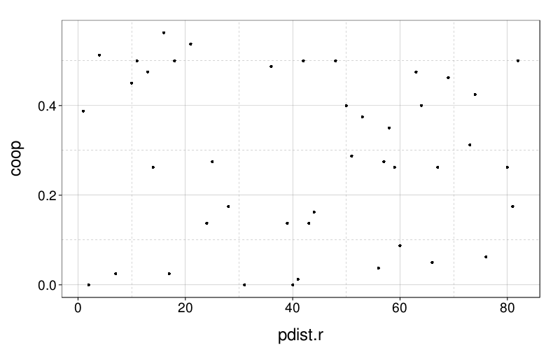
Apparently, there is no systematic relationship between pdist.r and cooperation rate:
ggplot(
    ddply(
        ss(ts, !(subject %in% bad.s) & !is.na(pdist.r) & show_opponent_score == "True"),
        .(pdist.r),
        function(slice) data.frame(coop = mean(slice$choice == "Cooperate")))) +
    geom_point(aes(pdist.r, coop))
Social-distance writeup
We computed social distance from the partner as follows. Within each subject, we fit a simple linear regression model with the subject's indifference value for persons #1, #2, #5, #10, #20, #50, and #100 as X and the integers 1 through 7 as Y. We also included another data point with X = 75 and Y = 0. Thus we attempted to robustly model the relationship between indifference amount (measured in dollars) and social distance (measured as rank within the list of person ranks 0, 1, 2, 5, 10, 20, 50, 100). Using the slope and intercept from this model and the indifference value for the partner, we computed the effective rank for the partner. Then we ranked these values across subjects to create our final measure of social distance from the partner.
To examine the effect of social distance from the partner on cooperation in the IPD, we fit a mixed-effects logistic regression model with a per-subject random effect and three fixed effects: one each for social distance from the partner, payoff matrix, and the opponent's choice. When fitting this model, we included only subjects in the social condition. This model, like the one described earlier, found that the 1-2-9-10 matrix and opponent cooperation significant increased subject cooperation (both zs > 4, both ps < .001). However, the effect of social distance from the partner was not significant (p = .741). Thus, we obtained no evidence that social distance from the partner influenced cooperation in the IPD.
Plots
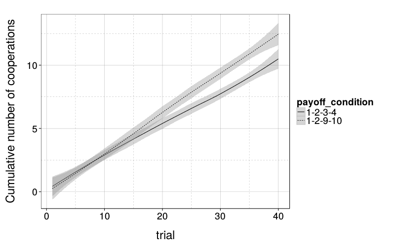
ggplot(ss(ts, show_opponent_score == "True")) +
    stat_smooth(aes(trial, cumcoop.n, linetype = payoff_condition), method = "loess", color = "black") +
    ylab("Cumulative number of cooperations")
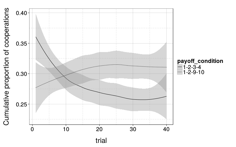
ggplot(ss(ts, show_opponent_score == "True")) +
    stat_smooth(aes(trial, cumcoop.p, linetype = payoff_condition), method = "loess", color = "black") +
    ylab("Cumulative proportion of cooperations")