Margin notebook

Delay (online only)

c("Sample size" = nlevels(ld.delay$s))

	value
Sample size	88

A plot of log-responses:

dodge(data = ld.delay, factor(dollars), log(mm), years)

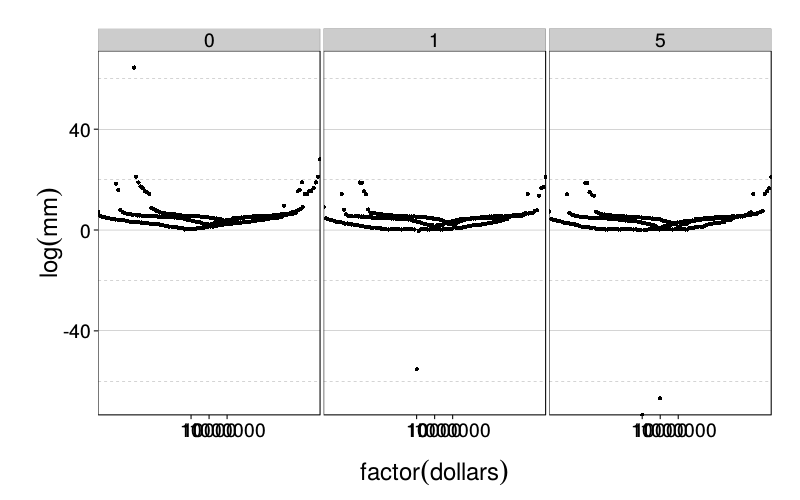
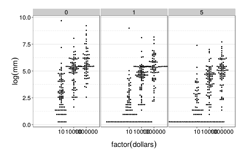
The discountinuous appearence of the distributions seem to arise from the choice of units. Here's a zoomed-in plot:

dodge(data = ss(ld.delay, log(mm) > 0 & log(mm) < 10),
    factor(dollars), log(mm), years)

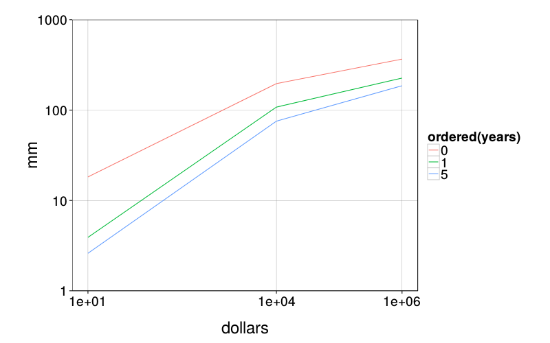
Between-subjects medians:

ggplot(ld.delay) +
    stat_summary(aes(dollars, mm, color = ordered(years)),
        fun.y = median, geom = "line") +
    scale_x_log10(breaks = c(1e1, 1e4, 1e6)) +
    scale_y_log10() +
    coord_cartesian(ylim = c(1, 1000)) +
    theme(panel.grid.minor = element_blank())

Now let's examine the significance of the interaction term in an appropriate statistical model.

model = lme(mm ~ dollars * years, random = ~1|s, data =
    transform(ld.delay,
        dollars = scale(log(dollars), scale = F),
        years = scale(years, scale = F),
        mm = log(pmax(1e-30, mm))))
rd(summary(model)$tTable[,"p-value"])

	value
(Intercept)	0.000
dollars	0.000
years	0.000
dollars:years	0.972

How about if we try the model with ranked millimeters?

model = lme(mm ~ dollars * years, random = ~1|s, data =
    transform(ld.delay,
        dollars = scale(log(dollars), scale = F),
        years = scale(years, scale = F),
        mm = rank(mm)))
rd(summary(model)$tTable[,"p-value"])

	value
(Intercept)	0.000
dollars	0.000
years	0.000
dollars:years	0.954

Still non-significant.

d = ss(dcast(
        ss(ld.delay,
            years %in% c(0, 1) & dollars %in% c(1e1, 1e4, 1e6),
            select = -trial),
        s ~ dollars + years,
        value.var = "mm"),
    `10_0` > `10_1` &
    `1000000_0` > `1000000_1` &
    `1000000_0` > `10_0` &
    `1000000_1` > `10_1`)
ratios = with(d,
    (log(`10_0`) - log(`10_1`)) /
    (log(`1000000_0`) - log(`1000000_1`)))
nrow(d)

	value
	61

table(ratios > 1)

	count
FALSE	13
TRUE	48

round(d = 5, t.test(log(ratios), mu = 0)$p.value)

	value
	0.00027

Significant (and in the right direction).

With the more extreme delay (5 years):

d = ss(dcast(
        ss(ld.delay,
            years %in% c(0, 5) & dollars %in% c(1e1, 1e4, 1e6),
            select = -trial),
        s ~ dollars + years,
        value.var = "mm"),
    `10_0` > `10_5` &
    `1000000_0` > `1000000_5` &
    `1000000_0` > `10_0` &
    `1000000_5` > `10_5`)
logratios = with(d,
    log(log(`10_0`) - log(`10_5`)) -
    log((log(`1000000_0`) - log(`1000000_5`))))
nrow(d)

	value
	68

table(logratios > 0)

	count
FALSE	21
TRUE	47

round(d = 5, t.test(pmin(10, logratios), mu = 0)$p.value)

	value
	0.00024

Also significant.

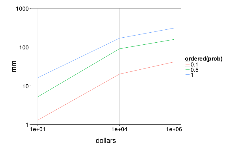
Probability

c("Sample size" = nlevels(ld.risk$s))

	value
Sample size	53

ggplot(ld.risk) +
    stat_summary(aes(dollars, mm, color = ordered(prob)),
        fun.y = median, geom = "line") +
    scale_x_log10(breaks = c(1e1, 1e4, 1e6)) +
    scale_y_log10() +
    coord_cartesian(ylim = c(1, 1000)) +
    theme(panel.grid.minor = element_blank())

d = ss(dcast(
        ss(ld.risk,
            prob %in% c(1, .5) & dollars %in% c(1e1, 1e4, 1e6),
            select = -trial),
        s ~ dollars + prob,
        value.var = "mm"),
    `10_1` > `10_0.5` &
    `1000000_1` > `1000000_0.5` &
    `1000000_1` > `10_1` &
    `1000000_0.5` > `10_0.5`)
ratios = with(d,
    (log(`10_1`) - log(`10_0.5`)) /
    (log(`1000000_1`) - log(`1000000_0.5`)))
nrow(d)

	value
	40

table(ratios > 1)

	count
FALSE	19
TRUE	21

rd(t.test(log(ratios), mu = 0)$p.value)

	value
	0.533

With the more extreme probability (.1):

d = ss(dcast(
        ss(ld.risk,
            prob %in% c(1, .1) & dollars %in% c(1e1, 1e4, 1e6),
            select = -trial),
        s ~ dollars + prob,
        value.var = "mm"),
    `10_1` > `10_0.1` &
    `1000000_1` > `1000000_0.1` &
    `1000000_1` > `10_1` &
    `1000000_0.1` > `10_0.1`)
ratios = with(d,
    (log(`10_1`) - log(`10_0.1`)) /
    (log(`1000000_1`) - log(`1000000_0.1`)))
nrow(d)

	value
	42

table(ratios > 1)

	count
FALSE	28
TRUE	14

rd(t.test(log(ratios), mu = 0)$p.value)

	value
	0.248

DMV function slopes

median.slopes = function(d)
   {names(d)[length(names(d)) - 1] = "trailer"
    d = ordf(d, s, dollars, trailer)
    d1 = ss(d, dollars == 10)
    d2 = ss(d, dollars == 1e4)
    d3 = ss(d, dollars == 1e6)
    do.call(rbind, lapply(sort(unique(d$trailer)), function(the.trailer)
       {d1t = ss(d1, trailer == the.trailer)
        d2t = ss(d2, trailer == the.trailer)
        d3t = ss(d3, trailer == the.trailer)
        slopes12 = (log(d2t$mm) - log(d1t$mm)) / (log(d2t$dollars) - log(d1t$dollars));
        slopes23 = (log(d3t$mm) - log(d2t$mm)) / (log(d3t$dollars) - log(d2t$dollars));
        data.frame(t = the.trailer,
            "1to2" = round(d = 3, median(slopes12)),
            "3to4" = round(d = 3, median(slopes23)))}))}

Below, the t column has the delay or probability and the next two columns have the slopes from $10 and $10k and $10k to $1M. These are medians of the slopes for individuals, but comparisons between cells would of course be between-subjects comparisons.

median.slopes(ld.delay)

	t	X1to2	X3to4
1	0	0.298	0.199
2	1	0.434	0.162
3	5	0.401	0.194

median.slopes(ld.risk)

	t	X1to2	X3to4
1	0.1	0.259	0.047
2	0.5	0.347	0.118
3	1.0	0.305	0.157

Slopes between across-subjects medians

logmm = with(ss(ld.delay, years == 0),
    tapply(log(mm), dollars, median))
rd(c(
    slope12 = num((logmm[2] - logmm[1]) / (log(1e4) - log(10))),
    slope23 = num((logmm[3] - logmm[2]) / (log(1e6) - log(1e4))),
    slope13 = num((logmm[3] - logmm[1]) / (log(1e6) - log(10))),
    b = num(coef(lm(y ~ x, data.frame(x = log(c(10, 1e4, 1e6)), y = num(logmm))))["x"])))

	value
slope12	0.344
slope23	0.136
slope13	0.261
b	0.267

Here slope12 is the slope of the line from $10 to $10k, slope23 is the the slope of the line from $10k to $1M, and slope13 is the slope of the line from $10 to $1M. b is the slope of the regression line for all three points.

Delay graph redo

medians.plot = function(sb, df, colname, label, point.size = 8, font.size = 14)
   {colnames(df)[colnames(df) == colname] = "x"
    d = data.frame(do.call(cbind, aggregate(mm ~ dollars + x,
        ss(df, s %in% row.names(sb)),
        function(v) quantile(v, c(.4, .5, .6)))))
    ggplot(d, aes(
            dollars * (1 + num(factor(x))/10 - .2),
            X50., ymin = X40., ymax = X60.)) +
        geom_line(aes(linetype = ordered(x))) +
        geom_point(size = point.size) +
        geom_linerange() +
        scale_x_log10(name = "amount (dollars)",
            breaks = c(1e1, 1e4, 1e6),
            labels = c("10", "10,000", "1 million")) +
        scale_y_log10(name = "happiness (mm)") +
        guides(linetype = guide_legend(title = label)) +
        coord_cartesian(ylim = c(1, 1000)) +
        theme_bw(base_size = font.size) + theme(
            panel.grid.minor = element_blank(),
            panel.grid.major = element_blank(),
            legend.position = c(1, 0), 
            legend.justification = c(1, 0),
            legend.background = element_rect(colour = "black", fill = "white"),
            panel.border = element_blank(),
            axis.line = element_line(color = "black"))}
medians.plot(sb, ld.delay, "years", "Delay (years)")

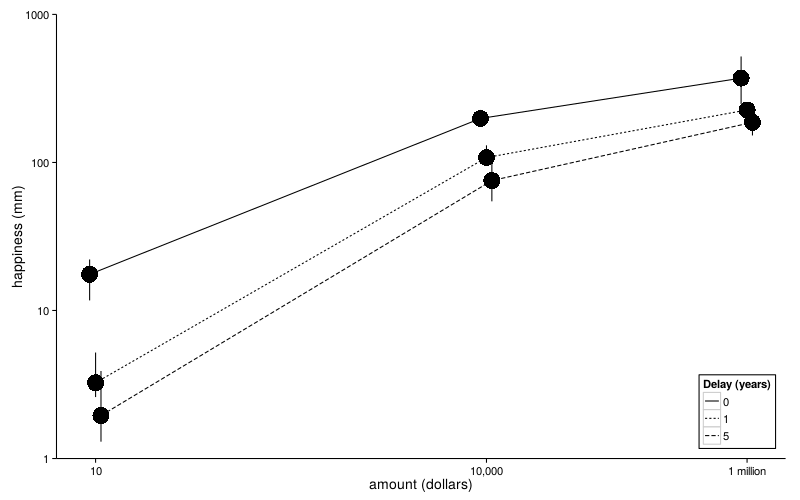
For generating the paper figure: cairo_ps("/tmp/out.eps", width = 6.5, height = 5); medians.plot(sb, ld.delay, "years", "Delay (years)", point.size = 2, font.size = 14); dev.off();