Philani notebook

Created 29 Sep 2016 • Last modified 8 Apr 2018

Previous studies

Retest of drinking during pregnancy

Reading notes

one

Ernhart, Morrow-Tlucak, Sokol, and Martier (1988) recruited 238 mothers from a Cleveland hospital and compared baseline (asking about drinking during the last 2 weeks at various points during pregnancy) to 5 years. They found that people more often went up than down (41% vs. 18%) but the proportion reporting no drinking was about the same at the two times (34% baseline vs. 36% later). Among sober at T1, 39% switched. Among drinkers at T1, 22% switched.
Jacobson, Chiodo, Sokol, and Jacobson (2002) recruited black mothers at a Detroit hospital, most of whom were recruited on the basis of drinking at conception, comparing during pregnancy to 13 months after birth. 59 mothers stated they abstained at baseline vs. 106 at follow-up. Mean absolute alcohol use per day was .23 at baseline vs. .88 at follow-up. "Among those who were inconsistent, 139 (61.8%) reported higher levels retrospectively, whereas only 86 (38.2%) report higher levels antenatally."
Hannigan et al. (2010) recruited black women from a Detroit hospital. "Among the 288 women, 43 (14.9%) reported more average drinking retrospectively (AAD) than they had previously reported antenatally" (and only 1 mother made the reverse change). Mean ounces of alcohol per day was .03 at baseline vs. .47 retrospectively. 284 mothers reporting abstaining or light drinking at baseline vs. 245 14 years after.
Alvik, Haldorsen, Groholt, and Lindemann (2006) recruited women from Oslo, Norway. "Questionnaires were answered at 17 (T1) and 30 weeks of pregnancy (T2) and 6 months after term (T3)." "Significantly more alcohol consumption after pregnancy recognition was reported retrospectively at both T2 and T3 [T2 0.15 and T3 0.18 standard units per week (SU/wk)] than concurrently at T1 or T2 (T1 0.10 and T2 0.14 SU/wk)." Reporting about T1, 24% of mothers reported any use at T1, 36% at T2, and 37% at T2. Specific within-subjects differences don't seem to be reported.

two

Ernhart et al. (1988): O'Connor and Paley (2006) says they "found that retrospective reports of drinking collected 5 years after pregnancy were more highly related to scores on a measure of alcohol-related problems and to craniofacial anomalies in children than were reports collected during pregnancy. Moreover, when questioned 5 years after the birth of their children, a large proportion of the women provided retrospective reports that were appreciably higher than those reports given while they were pregnant"
Jacobson et al. (2002): O'Connor and Paley (2006) says they "found reports of alcohol consumption taken during the antenatal period to be more highly associated with multiple measures of infant behavior at 13 months than retrospective reports of pregnancy drinking levels. Like Ernhart and associates (1988), they also found that retrospective recall yielded reports of higher levels of drinking than antenatal reports and that there was a statistically significant correlation between postpartum or current drinking and retrospective reports of consumption during pregnancy"
Hannigan et al. (2010): "Retrospective maternal self-reported drinking assessed 14 years postpartum was significantly higher than antenatal reports of consumption.… Retrospective report predicted more teen behavior problems (e.g., attention problems and externalizing behaviors) than the antenatal report."
Alvik et al. (2006): Oslo, Norway. "Questionnaires were answered at 17 (T1) and 30 weeks of pregnancy (T2) and 6 months after term (T3)." "Significantly more alcohol consumption after pregnancy recognition was reported retrospectively at both T2 and T3 [T2 0.15 and T3 0.18 standard units per week (SU/wk)] than concurrently at T1 or T2 (T1 0.10 and T2 0.14 SU/wk). When comparing the 2 retrospective reports at T2 and T3, there was a significant increase over time."

Analyses

Columns are contemporaneous and rows are retrospective.

Ernhart et al. (1988):

(setv ernhart-retest (pd.DataFrame
  :columns [4 3 2 1 0]
  :index [4 3 2 1 0]
  [
    [2  3  14  14  3]
    [0  0  7  8  2]
    [0  1  9  20  7]
    [0  0  5  38  20]
    [0  0  0  35  50]]))
(rd 2 [
  ["Proportion of T1 sober who were consistent"
    (/ (getl ernhart-retest 0 0)
      (.sum (getl ernhart-retest : 0)))]
  ["Proportion of T1 drinking who were consistent"
    (/ (.sum (.sum (getl ernhart-retest [4 3 2 1] [4 3 2 1])))
      (.sum (.sum (getl ernhart-retest : [4 3 2 1]))))]])

Proportion of T1 sober who were consistent	0.61
Proportion of T1 drinking who were consistent	0.78

Jacobson et al. (2002):

(setv jacobson-drink-cats (qw Very_Low Low Moderate Heavy Very_Heavy))
(setv jacobson-retest (pd.DataFrame
  :columns (+ ["Abstain"] jacobson-drink-cats)
  :index (+ ["Abstain"] jacobson-drink-cats)
  [
    [46  49  10  1  0  0]
    [7  45  17  2  0  0]
    [5  20  30  3  0  0]
    [0  9  25  2  3  0]
    [0  7  33  7  5  1]
    [1  2  9  8  6  1]]))
(rd 2 [
  ["Proportion of T1 sober who were consistent"
    (/ (getl jacobson-retest "Abstain" "Abstain")
      (.sum (getl jacobson-retest : "Abstain")))]
  ["Proportion of T1 drinking who were consistent"
    (/ (.sum (.sum (getl jacobson-retest jacobson-drink-cats jacobson-drink-cats)))
      (.sum (.sum (getl jacobson-retest : jacobson-drink-cats))))]])

Proportion of T1 sober who were consistent	0.78
Proportion of T1 drinking who were consistent	0.80

Hannigan et al. (2010):

(setv hannigan-retest (pd.DataFrame
  :columns (qw Abstain Lo)
  :index (qw Abstain Lo Mid Hi)
  [
    [222 3]
    [25 3]
    [14 0]
    [17 4]]))
(rd 2 [
  ["Proportion of T1 sober who switched"
    (/ (getl hannigan-retest "Abstain" "Abstain")
      (.sum (getl hannigan-retest : "Abstain")))]
  ["Proportion of T1 drinking who switched"
    (/ (.sum (.sum (getl hannigan-retest (qw Lo Mid Hi) "Lo")))
      (.sum (.sum (getl hannigan-retest : "Lo"))))]])

Proportion of T1 sober who switched	0.8
Proportion of T1 drinking who switched	0.7

Instrument and study design

Tom and Adriane's manuscripts can be found in \\CCHFS.semel.ucla.edu\Root\Projects & Programs\South Africa\PHILANI STUDY\FIVE YEAR ASSESSMENT\MANUSCRIPTS.

Use data up to the 5-year follow-up.

Some children were referred for FAS.

The timepoints are:

0: Baseline
1: Post birth (1-2 weeks)
2: 6 months
3: 18 months
4: 3 years
5: 5 years

Describe alcohol use over time, intervention vs. control. Alcohol use can be represented as any drinking or as our dichotomous problem-drinking measure.

Adriane: Looking at the surveys, I believe the alcohol questions were only asked of mothers. There are two variables for whether the mother drank any alcohol:
- alc_any: drank alcohol in the last month
- alc_any_a same as above, except for at time 1 (birth assessment), it is assigned a "1" if she drank in the last month and/or drank alcohol in the month prior to birth
alc_risk: see below

Child outcomes (as predicted by alcohol × intervention, and by whether the child is with the mother):

Fetal alcohol syndrome (FAS)
- Variables starting with FASD_ were only taken for children referred for FAS treatment; ref_need indicates need for a referral
- philtrum_rating, lip_rating: 4 or 5 indicates possible need for referral
CBCL
- First available at the year-3 followup. At year 5, only aggression items are available.
  - Aggressive_Behavior
Strengths & Difficulties
- First available at the year-3 followup. At year 5, only prosocial items are available.
  - Prosocial
Growth charts (weight for age, height for age)
- waz, haz, bmiz
Clancy Blair executive-function battery
- CSS_Sum - Silly Sounds (a Stroop-like task with cats and dogs)
- COS_Sum - Operation Span
- CSTS_Sum - Something's the Same
Kaufman IQ
- Kaufman_Standard_Score_MPI - only measured at timepoint 5

Variables with names ending with _1, _2, or _3 mean measurements of the first, second, and third child of a multiple birth.

Mary O'Connor says that Dawson, Grant, and Stinson (2005) is the right citation for our version of the AUDIT-C. In particular, that's where the threshold of 3 comes from. O'Connor et al. (2011) has the four items we used, which are the first two items from Dawson et al. (2005), plus two heavy-drinking items like the last item of Dawson et al., but with 4 and 3 drinks rather than 5. O'Connor et al. (2011) also says how to score each of the three items. The fact that Dawson et al.'s threshold of 3 might not be appropriate when using four rather than three items isn't addressed.

Mary O'Connor: "women are inclined to be more truthful about their drinking during that time [before recognizing their pregnancy] and… those data correlate most highly with cognitive deficits and physical dysmorphology"

Jackie Stewart: "The props [i.e., prop drink containers] we gave were a beer bottle, a wine glass (250mls) and a tot glass. Most of the participants were drinking cheap wine or beer." She confirmed that the goal of the props was to define "drink" for subjects in the sense of the American standard drink, which is 14 g of ethanol.

Mary O'Connor: "we ask about prior to pregnancy recognition drinking because mothers are supposedly more candid about that time period and because that measure predicts neurocognitive outcome better than during pregnancy results.… Prior to pregnancy recognition measures are important because most of the women booked very late in their pregnancies not finding out until much later than women from other countries and backgrounds so their prior to pregnancy recognition measures would include a large portion of their total gestational period."

Alcohol items, not about pregnancy

The number of the roughly equivalent AUDIT item is shown first.

(AUDIT 1) alc_freq (Absent at time 0) In the last month, about how often did you drink ANY alcoholic beverage?

Never [1]
Less than once a month [2]
Once a month [3]
2 to 3 times a month [4]
Once a week [5]
2 times a week [6]
3 to 4 times a week [7]
Nearly every day [8]
Every day [9]
Decline to answer [NA]

(AUDIT 2) alc_num (Absent at time 0) In the previous month before today, counting all types of alcohol combined, how many drinks did you USUALLY have on days when you drank alcohol?

1 or 2 [1]
3 or 4 [2]
5 or 6 [3]
7,8 or 9 [4]
10 or more [5]
Decline to answer [NA]

(AUDIT 3) alc_4_freq (Absent at time 0) In the previous month before today, about how often did you drink FOUR or MORE drinks in a single day?

Never [1]
Less than once a month [2]
Once a month [3]
2 to 3 times a month [4]
Once a week [5]
2 times a week [6]
3 to 4 times a week [7]
Nearly every day [8]
Every day [9]
Decline to answer [NA]

(AUDIT 6) alc_morning (Always present) Do you sometimes take a drink in the morning when you first get up?

Yes [1]
No [0]
Decline to answer [NA]

(Very roughly AUDIT 7) alc_cut_down (Always present) Do you sometimes feel the need to cut down on your drinking?

Yes [1]
No [0]
Decline to answer [NA]

(AUDIT 8) alc_memory (Always present) Has a friend or family member ever told you about things you said or did while you were drinking that you could not remember?

Yes [1]
No [0]
Decline to answer [NA]

(AUDIT 10) alc_friend (Always present) Have close friends or relatives worried or complained about your drinking?

Yes [1]
No [0]
Decline to answer [NA]

What we'll use: (wc dd (valcounts $time (& (>= $alc_4_freq 3) (>= (+ $alc_morning $alc_memory $alc_friend) 1)))) .

Alcohol items, about pregnancy

alc_freq_pre_b (Present only at time 0) How often did you use alcohol in the month before you found out you were pregnant?

Never [1]
Less than once a month [2]
Once a month [3]
2 to 3 times a month [4]
Once a week [5]
2 times a week [6]
3 to 4 times a week [7]
Nearly every day [8]
Every day [9]
Decline to answer [NA]

fas_alc_before (Present only at time 5) How often did you use alcohol in the month before you found out you were pregnant with [child]?

Never [1]
Less than once a month [2]
Once a month [3]
2 to 3 times a month [4]
Once a week [5]
2 times a week [6]
3 to 4 times a week [7]
Nearly every day [8]
Every day [9]
Decline to answer [NA]

alc_num_pre_b (Present only at time 0) During the month before you found out you were pregnant, counting all types of alcohol combined, how many drinks did you USUALLY have on days when you drank alcohol?

1 or 2 [1]
3 or 4 [2]
5 or 6 [3]
7,8 or 9 [4]
10 or more [5]
Decline to answer [NA]

fas_alc_per_day_before (Present only at time 5) During the month before you found out you were pregnant with [child] counting all types of alcohol combined, how many drinks did you USUALLY have on days when you drank alcohol?

1 or 2 [1]
3 or 4 [2]
5 or 6 [3]
7,8 or 9 [4]
10 or more [5]
Decline to answer [NA]

alc_freq_pre (Present only at timepoint 1) Within the last month, before your baby was born, about how often did you drink ANY alcoholic beverage?

Never [1]
Less than once a month [2]
Once a month [3]
2 to 3 times a month [4]
Once a week [5]
2 times a week [6]
3 to 4 times a week [7]
Nearly every day [8]
Every day [9]

alc_num_pre (Present only at timepoint 1) Within the last month, before your baby was born, counting all types of alcohol combined, how many drinks did you USUALLY have on days when you drank alcohol?

1 or 2 [1]
3 or 4 [2]
5 or 6 [3]
7,8 or 9 [4]
10 or more [5]

Pregnancies since the study pregnancy

Three relevant items are given_birth_since, pregnant_since_birth, and currently_preg. pregnant_since_birth appears at timepoints 3, 4, and 5. currently_preg appears at all these times as well as 2, but when pregnant_since_birth appears, a negative answer to it causes currently_preg to be skipped.

pregnant_since_birth Have you been pregnant again since the birth of [child]? (Recoded to 0/1 in the Philani combo file.)

Yes [1]
No [2]

currently_preg Are you currently pregnant? [INTERVIEWER: DO NOT READ OUT THE LIST PRESENTED HERE, PLEASE LISTEN TO WHAT THE MOTHER TELLS YOU AND THEN TICK ONE OPTION]

Yes [1]
No [2]
I was but I miscarried [3]
I was but I had an abortion [4]
Decline to answer [91]

Comparing pregnant_since_birth to currently_preg, it seems that we capture only a minority of pregnancies with currently_preg, which is plausible given how large the intervals between assessments are at the later timepoints.

Note that consistency over timepoints in the subject's responses to pregnant_since_birth wasn't enforced.

Deaths

Deaths of mothers and children are recorded in DEATHS&ADVERSE EVENTS_Philani Study_updated.xlsx. Ellen explains that the "Death Time" column is to be interpreted as meaning that the death occurred between the corresponding timepoint and the next; e.g., Death Time 0 means that the mother or child died between timepoints 0 and 1.

Data

Except where otherwise noted, analyses of drinking data use the baseline items asking mothers about after they'd noticed they were pregnant, and the after-birth items asking mothers about after they gave birth. This is because follow-up questions that I use to identify problem drinking weren't asked about the other sub-timepoints queried about at these timepoints, namely, before the mother noticed she was pregnant at the baseline timepoint, and before birth at the after-birth timepoint.

Follow-up rate among baseline mothers

(setv s-baseline (ss obs (= $timepoint "Baseline") "s"))
(setv df-followup (.apply (.groupby (ss obs (.isin $s s-baseline)) "timepoint")
  (λ (pds-from-pairs [
    ["n" (len it)]
    ["mean_days" (.mean ($ it child_age_days))]
    ["sd_days" (np.std ($ it child_age_days))]]))))
(rd 1 df-followup)

timepoint	n	mean_days	sd_days
Baseline	1144	-81.2	54.2
After_birth	1058	13.5	14.9
6_months	1007	189.7	22.8
18_months	953	561.2	42.1
3_years	872	1111.9	65.8
5_years	844	1881.6	99.1

(defn f [timepoint unit-name unit-divisor]
  [timepoint
    (rd 2 (/ (getl df-followup timepoint "n") (len s-baseline)))
    (+ (str (rd 1 (/ (getl df-followup timepoint "mean_days") unit-divisor)))
      " " unit-name)
    (+ (str (rd 1 (/ (getl df-followup timepoint "sd_days") unit-divisor)))
      " " unit-name)])

(pd.DataFrame :columns (qw timepoint returned mean_time sd_time) [
  (f "After_birth" "days" 1)
  (f "6_months" "months" 30.436875)
  (f "18_months" "months" 30.436875)
  (f "3_years" "years" 365.2425)
  (f "5_years" "years" 365.2425)])

I	timepoint	returned	mean_time	sd_time
0	After_birth	0.92	13.5 days	14.9 days
1	6_months	0.88	6.2 months	0.7 months
2	18_months	0.83	18.4 months	1.4 months
3	3_years	0.76	3.0 years	0.2 years
4	5_years	0.74	5.2 years	0.3 years

(setv g (.groupby (ss obs (.isin $s s-baseline)) "s"))
[
  ["Appeared at all timepoints" (rd 3 (.mean (.apply g (λ (= (len it) 6)))))]
  ["Never reassessed" (rd 3 (.mean (.apply g (λ (= (len it) 1)))))]]

Appeared at all timepoints	0.702
Never reassessed	0.071

Old follow-up numbers

Here are the computations that replicate the sample sizes obtained by Ellen and Panteha for their flowchart. A "death" is a mother who died or whose child died (or both).

(setv d (ss obs (= $condition "Control")))
(concat (rmap [tp (. ($ d timepoint) cat categories)] [
  [(.format "Mothers at {}, plus anachronistic late entries" tp)
    (+
      (.sum (wc d (= $timepoint tp)))
      (.sum (.apply (.groupby d "s") (λ
        (.all (> ($ it timepoint) tp))))))]
  [(.format "All mothers minus deaths before {}" tp)
    (- (len (.unique ($ d s)))
      (.sum (wc d (& $death (< $timepoint tp)))))]
  [NaN NaN]
  [(.format "Deaths between {} and the next timepoint" tp)
    (len (ss d (& (= $timepoint tp) $death)))]]))

Mothers at Baseline, plus anachronistic late entries	594
All mothers minus deaths before Baseline	594

Deaths between Baseline and the next timepoint	41
Mothers at After_birth, plus anachronistic late entries	546
All mothers minus deaths before After_birth	553

Deaths between After_birth and the next timepoint	7
Mothers at 6_months, plus anachronistic late entries	509
All mothers minus deaths before 6_months	546

Deaths between 6_months and the next timepoint	5
Mothers at 18_months, plus anachronistic late entries	496
All mothers minus deaths before 18_months	541

Deaths between 18_months and the next timepoint	4
Mothers at 3_years, plus anachronistic late entries	455
All mothers minus deaths before 3_years	537

Deaths between 3_years and the next timepoint	2
Mothers at 5_years, plus anachronistic late entries	443
All mothers minus deaths before 5_years	535

Deaths between 5_years and the next timepoint	0

This table is for the controls. "Anachronistic late entries" are mothers who entered the study later than than the indicated timepoint.

(setv d (ss obs (= $condition "Mentor_Mother")))
(concat (rmap [tp (. ($ d timepoint) cat categories)] [
  [(.format "Mothers at {}" tp)
    (.sum (wc d (= $timepoint tp)))]
  [(.format "All mothers minus deaths before {}" tp)
    (- (len (.unique ($ d s)))
      (.sum (wc d (& $death (< $timepoint tp)))))]
  [NaN NaN]
  [(.format "Deaths between {} and the next timepoint" tp)
    (len (ss d (& (= $timepoint tp) $death)))]]))

Mothers at Baseline	644
All mothers minus deaths before Baseline	644

Deaths between Baseline and the next timepoint	28
Mothers at After_birth	606
All mothers minus deaths before After_birth	616

Deaths between After_birth and the next timepoint	11
Mothers at 6_months	573
All mothers minus deaths before 6_months	605

Deaths between 6_months and the next timepoint	10
Mothers at 18_months	543
All mothers minus deaths before 18_months	595

Deaths between 18_months and the next timepoint	11
Mothers at 3_years	497
All mothers minus deaths before 3_years	584

Deaths between 3_years and the next timepoint	6
Mothers at 5_years	477
All mothers minus deaths before 5_years	578

Deaths between 5_years and the next timepoint	2

This table is for the mentored subjects. All late-entry mothers were put in the control condition, so we don't have to worry about late entries here.

Here's some text I wrote using the above numbers:

Pregnant women over the age of 18 years old were initially recruited to the study from May 2009 until September 2010 by township women; only 2% of those approached declined to participate. Recruiters visited each household monthly to find pregnant women during this period. There were five follow-up timepoints: approximately 2 weeks after the birth of the child (mean duration 13.5 days, SD 14.9 days), 6 months (mean 6.2 months, SD 0.7 months), 18 months (mean 18.4 months, SD 1.4 months), 3 years (mean 3.0 years, SD 0.2 years), and 5 years (mean 5.2 years, SD 0.3 years).

There was a total of 594 control mothers, including 94 mothers ("late entries") who were recruited after baseline: 19 mothers at the after-birth timepoint, 53 at 6 months, and 22 at 18 months. There were 41 deaths (of a mother, her child, or both) before the after-birth timepoint, leaving 553 subjects; the number who were assessed at this timepoint plus the number of future late entries is 546 (99%). Before 6 months, there were 7 more deaths, leaving 546 subjects; the number assessed at 6 months plus future late entries is 509 (93%). Before 18 months, there were 5 more deaths, leaving 541 subjects, 496 of whom were assessed (92%). Before 3 years, there were 4 more deaths, leaving 537 subjects, 455 of whom were assessed (85%). Before 5 years, there were 2 more deaths, leaving 535 subjects, 443 of whom were assessed (83%).

There was a total of 644 mentored mothers, all of whom were assessed at baseline. There were 28 deaths after the after-birth timepoint, leaving 616 subjects, 606 of whom were assessed at this timepoint (98%). Before 6 months, there were 11 more deaths, leaving 605 subjects, 573 of whom were assessed (95%). Before 18 months, there were 10 more deaths, leaving 595 subjects, 543 of whom were assessed (91%). Before 3 years, there were 11 more deaths, leaving 584 subjects, 497 of whom were assessed (85%). Before 5 years, there were 6 more deaths, leaving 578 subjects, 477 of whom were assessed (83%).

Drinking

Figures

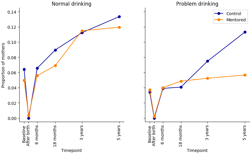
(setv d (.dropna (getl obs : (qw condition timepoint alcohol_state))))
(setv ($ d Normal) (= ($ d alcohol_state) "Okay"))
(setv ($ d Problem) (= ($ d alcohol_state) "Problem"))
(setv d (pd.melt d (qw condition timepoint) (qw Normal Problem)))
(sns.factorplot "timepoint" "value" :hue "condition" :col "variable"
  :data d :ci None :legend F :size 6)
(plt.legend :loc "best")

(rd (.apply
  (wc
    (.dropna (ss obs (= $timepoint "5_years")
      (qw alcohol_state condition)))
    (valcounts $alcohol_state $condition))
  (λ (/ it (.sum it)))))

alcohol_state	Control	Mentor_Mother
Sober	0.753	0.824
Okay	0.133	0.119
Problem	0.113	0.057

This table shows the proportion of mothers in each condition and drinking state at 5 years. Mothers in the mentored group are problem drinkers at half the rate as in control.

(setv d (.dropna (getl obs :
  (qw s condition timepoint alcohol_any alcohol_problem))))
(setv ($ d alcohol_state) (.astype (wc d
  (np.where (= $alcohol_any "Sober")    0
  (np.where (= $alcohol_problem "Okay") 1
                                        2))) float))
(setv d (.dropna (.pivot d "s" "timepoint" "alcohol_state")))
(setv d (get (ordf d (.sum d :axis 1) $Baseline $After_birth $6_months $18_months $3_years $5_years)
  (.any d :axis 1)))
(sns.heatmap d :cbar F)

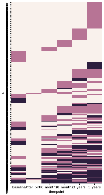
This lasagna plot isn't very useful, but it shows each mother's state (light for non-drinking, pink for non-problem drinking, and dark for problem drinking) at each timepoint. Each mother is a row. Mothers who never drank are excluded from this plot.

Mixed-effects ordinal regression

I fit a mixed-effects ordinal probit-regression model, with per-subject random intercepts. The DV is a 3-valued ordinal variable where the lowest level is not drinking (Sober), the intermediate level is non-problem drinking (Okay), and the highest level is problem drinking (Problem). The IVs are timepoint and condition. I exclude the After_birth timepoint since almost nobody drank then.

(setv alc-ordinal-results (cache "alc-ordinal" (fn [] (R-call
  "function(d)
      {d$alcohol_state = ordered(d$alcohol_state)
       library(ordinal)
       set.seed(10)
       m = clmm(alcohol_state ~ condition * timepoint + (1|s),
           data = d, link = 'probit', nAGQ = 7)
       x = coef(summary(m))[,'Estimate']
       list(nrow(d), length(unique(d$s)), names(x), cbind(x, confint(m)))}"
  (drop-unused-cats (.dropna
    (ss obs (!= $timepoint "After_birth")
      (qw s condition timepoint alcohol_state))))))))
1

Retest of drinking during pregnancy

Any or none

(setv pregdrink-retest (.pivot
  (ss obs (.isin $timepoint (qw Baseline 5_years)))
  "s" "timepoint" "alcohol_any_preg_before_noticed"))
(setv pregdrink-retest (.astype pregdrink-retest {"Baseline" object "5_years" object}))
  ; This works around a pandas bug that would otherwise cause the
  ; next statement to fail.
(setv ($ pregdrink-retest condition)
  (getl conditions pregdrink-retest.index))

[
  ["subjects responding at 1 or both timepoints"
    (.sum (wc pregdrink-retest (| (pd.notnull $Baseline) (pd.notnull $5_years))))]
  ["subjects responding at both timepoints"
    (.sum (wc pregdrink-retest (& (pd.notnull $Baseline) (pd.notnull $5_years))))]
  ["subjects responding at baseline"
    (.sum (pd.notnull ($ pregdrink-retest Baseline)))]
  ["subjects reporting drinking at baseline"
    (.sum (= ($ pregdrink-retest Baseline) "Drinking"))]
  ["proportion" (rd 2 (/
    (.sum (= ($ pregdrink-retest Baseline) "Drinking"))
    (.sum (pd.notnull ($ pregdrink-retest Baseline)))))]
  ["subjects responding at 5 years"
    (.sum (pd.notnull ($ pregdrink-retest 5_years)))]
  ["subjects reporting drinking at 5 years"
    (.sum (= ($ pregdrink-retest 5_years) "Drinking"))]
  ["proportion" (rd 2 (/
    (.sum (= ($ pregdrink-retest 5_years) "Drinking"))
    (.sum (pd.notnull ($ pregdrink-retest 5_years)))))]
  ["proportion of subjects with concordant responses" (rd 2
    (.mean (wc (.dropna pregdrink-retest) (= $Baseline $5_years))))]
]

subjects responding at 1 or both timepoints	1220.00
subjects responding at both timepoints	843.00
subjects responding at baseline	1144.00
subjects reporting drinking at baseline	284.00
proportion	0.25
subjects responding at 5 years	919.00
subjects reporting drinking at 5 years	174.00
proportion	0.19
proportion of subjects with concordant responses	0.85

(rmap [[timepoint condition] (product (qw Baseline 5_years) (qw Control Mentor_Mother))]
  [(.format "proportion drinking: {}, {}" timepoint condition)
    (rd 2 (.mean (= "Drinking" (.dropna
      (getl (ss pregdrink-retest (= $condition condition)) : timepoint)))))])

proportion drinking: Baseline, Control	0.26
proportion drinking: Baseline, Mentor_Mother	0.24
proportion drinking: 5_years, Control	0.21
proportion drinking: 5_years, Mentor_Mother	0.17

condition	Baseline	Drinking	Sober	prop
Control	Drinking	56	33	0.63
Control	Sober	23	254	0.08
Mentor_Mother	Drinking	60	51	0.54
Mentor_Mother	Sober	22	344	0.06

Here's a within-subjects point of view. The columns "Drinking" and "Sober" are 5-year responses. In both conditions, subjects who said sober at baseline were very likely to say the same later, whereas subjects who said drinking at baseline had a fair likelihood of switching to sober.

Amounts

(setv pregdrink-retest-amnt (.pivot
  (ss obs (.isin $timepoint (qw Baseline 5_years)))
  "s" "timepoint" "alcohol_aa/day_preg_before_noticed"))
(setv pregdrink-retest-amnt (.astype pregdrink-retest-amnt {}))
  ; This works around a pandas bug that would otherwise cause the
  ; next statement to fail.
(setv ($ pregdrink-retest-amnt condition)
  (getl conditions pregdrink-retest-amnt.index))

(setv d pregdrink-retest-amnt  both (.dropna pregdrink-retest-amnt))

[
  ["subjects responding at 1 or both timepoints"
    (.sum (wc d (| (pd.notnull $Baseline) (pd.notnull $5_years))))]
  ["subjects responding at both timepoints"
    (.sum (wc d (& (pd.notnull $Baseline) (pd.notnull $5_years))))]
  ["proportion increasing" (rd 2
    (.mean (wc both (> $5_years $Baseline))))]
  ["proportion decreasing" (rd 2
    (.mean (wc both (< $5_years $Baseline))))]
  ["proportion with no change" (rd 2
    (.mean (wc both (= $5_years $Baseline))))]
  ["mean change" (rd 2
    (.mean (wc both (- $5_years $Baseline))))]]

subjects responding at 1 or both timepoints	1220.00
subjects responding at both timepoints	842.00
proportion increasing	0.16
proportion decreasing	0.13
proportion with no change	0.72
mean change	0.07

(plt.clf)
(plt.axis "equal")
(plt.plot [0 3] [0 3] :c "black" :linewidth .5 :zorder -3)
(defn jitter [v]
  (+ v (* (- (np.random.random (len v)) .5) .05)))
(wc (.dropna pregdrink-retest-amnt)
  (plt.scatter (jitter $Baseline) (jitter $5_years) :s 1))

RMSE comparison (no CV)

(import [statsmodels.api :as sm])

(defn rmse [v1 v2]
  (np.sqrt (np.mean (** (- v1 v2) 2))))

(defn pred-dichot [df xv yv]
  (setv means (.mean (.groupby (getl df : [xv yv]) xv)))
  (setv y-pred (getl means (getl df : xv) yv))
  (rmse (. (getl df : yv) values) y-pred.values))

(defn pred-amnt [df xv yv]
  (setv m (sm.OLS
    (. (getl df : yv) values)
    (sm.add-constant (. (.astype (getl df : xv) float) values))))
  (setv y-pred (.predict (.fit m)))
  (rmse (. (getl df : yv) values) y-pred))

(defn pred-amnt-hinged [df xv yv]
  (setv x (. (.astype (getl df : xv) float) values))
  (setv m (sm.OLS
    (. (getl df : yv) values)
    (np.column-stack [
      (sm.add-constant x)
      (!= x 0)])))
  (setv y-pred (.predict (.fit m)))
  (rmse (. (getl df : yv) values) y-pred))

(setv [d-dichot d-amnt] (rmap [d [pregdrink-retest pregdrink-retest-amnt]]
  (.dropna (.merge (.reset-index d)
    (ss obs (= $timepoint "5_years") ["s" "child_kaufman_iq"])))))
(setv v (rd (pds-from-pairs :name "RMSE" [
  ["Baseline (SD)" (wc d-dichot (.std $child_kaufman_iq :ddof 0))]
  ["T1, dichotomous" (pred-dichot d-dichot "Baseline" "child_kaufman_iq")]
  ["T1, continuous" (pred-amnt d-amnt "Baseline" "child_kaufman_iq")]
  ["T1, hinged" (pred-amnt-hinged d-amnt "Baseline" "child_kaufman_iq")]
  ["T2, dichotomous" (pred-dichot d-dichot "5_years" "child_kaufman_iq")]
  ["T2, continuous" (pred-amnt d-amnt "5_years" "child_kaufman_iq")]
  ["T2, hinged" (pred-amnt-hinged d-amnt "5_years" "child_kaufman_iq")]])))
(setv v.index.name "Model")
v

Table 1. Accuracy of "predicting" year-5 child IQ using measures of drinking during pregnancy taken at baseline (T1) or 5 years after the child's birth (T2), and using dichotomous (drinking or not drinking) or continuous (fluid ounces of absolute alcohol per day) coding. RMSE = root mean square error
Model	RMSE
Baseline (SD)	11.301
T1, dichotomous	11.286
T1, continuous	11.285
T1, hinged	11.273
T2, dichotomous	11.297
T2, continuous	11.290
T2, hinged	11.287

CV

(defn rmse [v1 v2]
  (np.sqrt (np.mean (** (- v1 v2) 2))))

(defn pred-ols [x y cv-obj]
  (np.sqrt (- (np.mean (sklearn.model-selection.cross-val-score
    (sklearn.linear-model.LinearRegression :fit-intercept T)
    x y
    :scoring "neg_mean_squared_error" :cv cv-obj)))))
(defn pred-nothing [df yv cv-obj]
  (setv y (. (getl df : yv) values))
  (setv y-pred (np.array (rmap [[i-train i-test] cv-obj]
    (np.mean (geta y i-train)))))
  (rmse y y-pred))
(defn pred-dichot [df xv yv cv-obj]
  (pred-ols
    (.reshape (. (= (getl df : xv) "Drinking") values) -1 1)
    (. (getl df : yv) values)
    cv-obj))
(defn pred-amnt [df xv yv cv-obj]
  (pred-ols
    (.reshape (. (.astype (getl df : xv) float) values) -1 1)
    (. (getl df : yv) values)
    cv-obj))

(setv d (rd (pd.concat :axis 1 (rmap [[colname yv y-timepoint] [
    ["Head circumference" "child_head_circumference_for_age_z" "After_birth"]
    ["Intelligence" "child_kaufman_iq" "5_years"]]]
  (setv [d-dichot d-amnt] (rmap [d [pregdrink-retest pregdrink-retest-amnt]]
    (setv d (.dropna (.merge (.reset-index d) (ss obs
      (& (= $condition "Control") (= $timepoint y-timepoint))
      ["s" yv]))))
    (.set-index (getl d : ["s" "Baseline" "5_years" yv]) "s")))
  (assert (.issubset (set d-amnt.index) (set d-dichot.index)))
  (setv d-dichot (getl d-dichot d-amnt.index))
  (setv cv-obj (list (.split (sklearn.model-selection.LeaveOneOut) d-dichot)))
  (pds-from-pairs :name colname [
    ["(Sample size)" (str (len d-dichot))]
    ["Baseline (constant only)" (pred-nothing d-dichot yv cv-obj)]
    ["T1, dichotomous" (pred-dichot d-dichot "Baseline" yv cv-obj)]
    ["T1, continuous" (pred-amnt d-amnt "Baseline" yv cv-obj)]
    ["T2, dichotomous" (pred-dichot d-dichot "5_years" yv cv-obj)]
    ["T2, continuous" (pred-amnt d-amnt "5_years" yv cv-obj)]])))))
(setv d.index.name "Model")
d

Table 2. Accuracy (as root mean square error) of predicting head circumference after birth (WHO `z`-score for age and sex) and year-5 child intelligence (Kaufman mental processing index; MPI) using measures of drinking during pregnancy taken at baseline (T1) or 5 years after the child's birth (T2), and using dichotomous (drinking or not drinking) or continuous (fluid ounces of absolute alcohol per day) coding.
Model	Head circumference	Intelligence
(Sample size)	364	284
Baseline (constant only)	1.847	11.057
T1, dichotomous	1.847	11.070
T1, continuous	1.847	11.120
T2, dichotomous	1.848	11.061
T2, continuous	1.839	11.086

Weight and height at birth

(rectplot :diam .1 ($ obs child_birthweight_kg))

(rectplot ($ obs child_birthheight_cm))

This should be capped around 60.

Head circumference-for-age z-scores

(rectplot :diam .1 (ss obs (= $timepoint "After_birth")
  "child_head_circumference_for_age_z"))

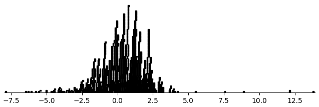
Weight-for-age and height-for-age z-scores

(setv aics (alc-model-aics "child_weight_for_age_z" "normal"))
(show-alc-model-aics aics)

I	value
n_obs	3374
n_subjects	1003
n_timepoints	4
no_alc	8894
prenatal	8890
current	8889
both	8887

The model with all alcohol terms has the least AIC.

(.round (alc-model-coefcis "both" "child_weight_for_age_z" "normal") 2)

Coefficient	Low	Point	High
6 months	0.47	0.58	0.69
18 months	0.15	0.27	0.39
3 years	-0.05	0.06	0.17
5 years	-0.11	0.02	0.15
Mentored × 6 months	-0.25	-0.09	0.08
Mentored × 18 months	-0.09	0.06	0.23
Mentored × 3 years	-0.12	0.03	0.19
Mentored × 5 years	-0.16	0.02	0.18
Prenatal normal drinking	-0.30	0.07	0.50
Prenatal problem drinking	-0.91	-0.31	0.19
Current normal drinking	-0.22	-0.08	0.07
Current problem drinking	-0.42	-0.21	-0.02
Mentored × Prenatal normal drinking	-1.17	-0.63	-0.07
Mentored × Prenatal problem drinking	-0.50	0.14	0.87
Mentored × Current normal drinking	-0.17	0.03	0.22
Mentored × Current problem drinking	-0.35	-0.05	0.21

At 6 months, the children are unusually fat, half a z-score more than the mean on average. The average diminishes to be a little fatter than typical at 18 months and typical at 3 years and 5 years. The intervention has little effect at each timepoint, with suggestions of a negative effect at 6 months and a positive effect at 18 months.

prenatal_alc_Okay - unknown
prenatal_alc_Problem - highly uncertain, with weight of evidence towards a moderate negative effect
alc_Okay - perhaps small negative effect
alc_Problem - negative effect of up to moderate size
Mentor_Mother × prenatal_alc_Okay - negative effect of unknown size, with weight of evidence towards very strong
Mentor_Mother × prenatal_alc_Problem - unknown
Mentor_Mother × alc_Okay - small effect of unknown direction
Mentor_Mother × alc_Problem - small effect of unknown direction

To summarize the alcohol effects, they are uncertain but tend towards the negative. Oddly, the intervention worsens the effect of normal prenatal drinking.

(setv aics (alc-model-aics "child_height_for_age_z" "normal"))
(show-alc-model-aics aics)

I	value
n_obs	3370
n_subjects	1003
n_timepoints	4
no_alc	10412
prenatal	10410
current	10417
both	10415

The model with prenatal alcohol has the least AIC.

(.round (alc-model-coefcis "prenatal" "child_height_for_age_z" "normal") 2)

Coefficient	Low	Point	High
6 months	-0.39	-0.27	-0.15
18 months	-0.77	-0.62	-0.49
3 years	-1.55	-1.40	-1.26
5 years	-0.74	-0.60	-0.48
Mentored × 6 months	0.00	0.17	0.33
Mentored × 18 months	-0.08	0.08	0.26
Mentored × 3 years	-0.13	0.05	0.25
Mentored × 5 years	-0.12	0.05	0.22
Prenatal normal drinking	-0.11	0.28	0.66
Prenatal problem drinking	-0.98	-0.47	0.05
Mentored × Prenatal normal drinking	-1.05	-0.56	0.00
Mentored × Prenatal problem drinking	-0.55	0.17	0.78

The children are shorter than normal, especially at age 3.

prenatal_alc_Okay - uncertain, leaning towards moderately positive
prenatal_alc_Problem - negative of unknown size, possibly quite strong
Mentor_Mother × prenatal_alc_Okay - negative of uncertain size, possibly quite strong
Mentor_Mother × prenatal_alc_Problem - uncertain, leaning towards positive

To summarize, normal prenatal drinking may have a positive effect, whereas problem prenatal drinking has a negative effect. As in the previous model, the intervention worsens the effect of normal prenatal drinking.

Bayley tests

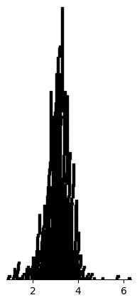
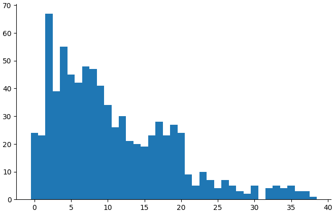
(density-plot (.dropna ($ obs child_bayley_cognitive)))

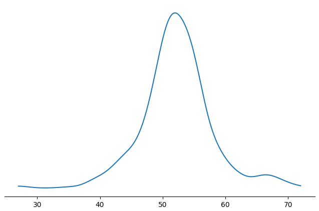
A nice distribution.

(setv v (sorted (.dropna ($ obs child_bayley_motor))))
[(cut v 0 10) (cut v -10)]

8	35	36	40	41	44	44	45	45	46
59	60	60	60	60	60	61	61	64	80

The motor subscale has a very extreme value on each end. Let's clip to second-most-extreme values.

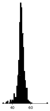
(density-plot (.clip (.dropna ($ obs child_bayley_motor)) 35 64))

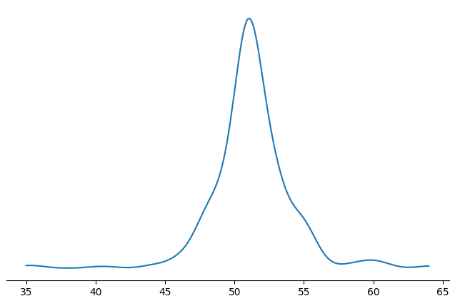
Better.

Kaufman IQ

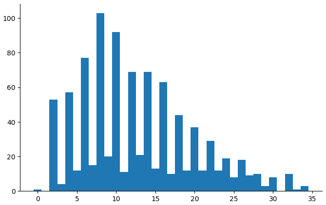
(rectplot (.dropna ($ obs child_kaufman_iq)))

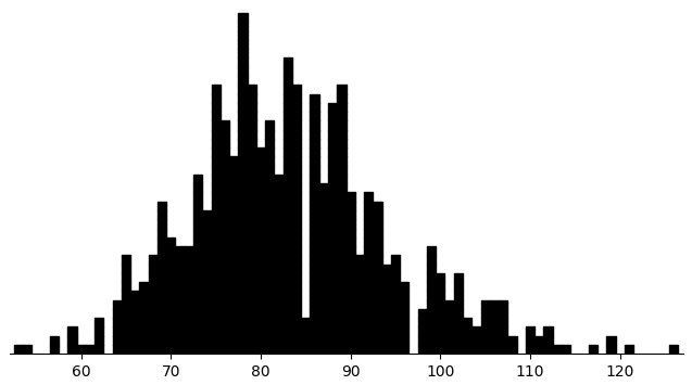
Here there's only one timepoint, so we can use a fairly simple OLS model.

(setv aics (alc-model-aics "child_kaufman_iq" "normal"))
(show-alc-model-aics aics)

I	value
n_obs	646
n_subjects	646
n_timepoints	1
no_alc	4973
prenatal	4976
current	4981
both	4984

Surprisingly, the alcohol terms don't help.

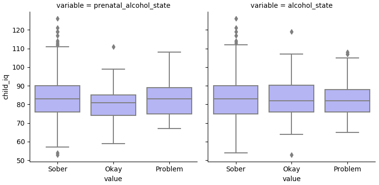
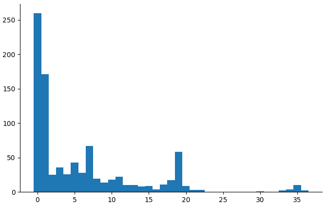
(alc-outcome-plot "child_kaufman_iq")

CBCL: Aggression

(countbars "child_cbcl_aggress" "3_years")

(countbars "child_cbcl_aggress" "5_years")

At 3 years, mothers were heavily biased against rating items 1, but it doesn't look like there's much I can do about this. At 5 years, the distribution looks decent.

Strengths & Difficulties: Prosocial

(setv v (.value-counts ($ obs child_sdq_prosocial)))
(plt.bar v.index v)

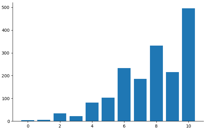
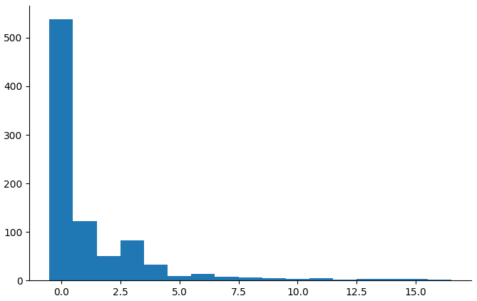
This measure seems to be subject to a ceiling effect, so relationships of it with anything else will be hard to find.

(setv aics (alc-model-aics "child_sdq_prosocial" "normal"))
(show-alc-model-aics aics)

I	value
n_obs	1567
n_subjects	879
n_timepoints	2
no_alc	6702
prenatal	6706
current	6705
both	6707

Indeed, the alcohol terms don't help.

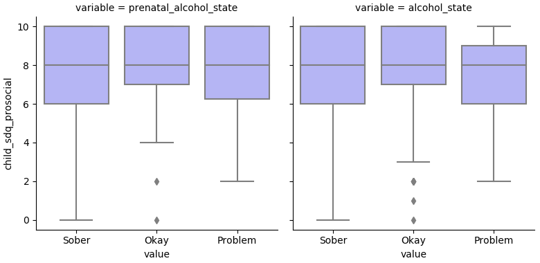
(alc-outcome-plot "child_sdq_prosocial")

Clancy Blair executive-function battery

Silly Sounds

(countbars "child_execufun_silly_sounds" "3_years")

(countbars "child_execufun_silly_sounds" "5_years")

This measure has a floor effect at 3 years and a severe ceiling effect at 5 years.

(setv aics (alc-model-aics "child_execufun_silly_sounds" "binomial"))
(show-alc-model-aics aics)

I	value
n_obs	1545
n_subjects	866
n_timepoints	2
no_alc	9632
prenatal	9634
current	9614
both	9615

Surprisingly, alcohol helps. We'll use the current model, since current drinking seems to help a lot more than prenatal drinking.

(.round (alc-model-coefcis "current" "child_execufun_silly_sounds" "binomial") 1)

Coefficient	Low	Point	High
3 years	-2.6	-2.4	-2.2
5 years	3.5	3.7	4.0
Current normal drinking	-0.2	0.2	0.6
Current problem drinking	-1.5	-1.1	-0.6
Mentored × 3 years	-0.3	-0.0	0.2
Mentored × 5 years	-0.4	-0.1	0.2
Mentored × Current normal drinking	-0.5	0.1	0.6
Mentored × Current problem drinking	0.6	1.3	2.0

Problem alcohol use substantially lowers Silly Sounds scores, but the intervention undoes this.

Operation Span

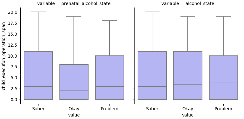
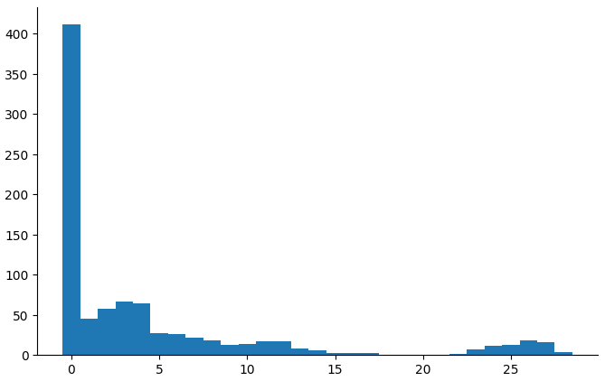
(countbars "child_execufun_operation_span" "3_years")

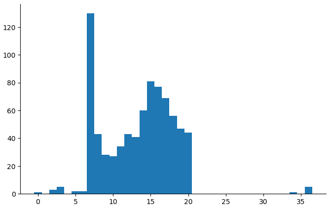
(countbars "child_execufun_operation_span" "5_years")

At 3 years, but not at 5 years, the measure has a severe floor effect.

(setv aics (alc-model-aics "child_execufun_operation_span" "binomial"))
(show-alc-model-aics aics)

I	value
n_obs	1545
n_subjects	866
n_timepoints	2
no_alc	7866
prenatal	7871
current	7873
both	7878

Alcohol doesn't help.

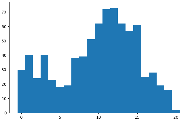
(alc-outcome-plot "child_execufun_operation_span")

Something's the Same

(countbars "child_execufun_something_same" "3_years")

(countbars "child_execufun_something_same" "5_years")

This one has a floor at 3 years and a spike at 5 years.

References

Alvik, A., Haldorsen, T., Groholt, B., & Lindemann, R. (2006). Alcohol consumption before and during pregnancy comparing concurrent and retrospective reports. Alcoholism, 30(3), 510–515. doi:10.1111/j.1530-0277.2006.00055.x

Dawson, D. A., Grant, B. F., & Stinson, F. S. (2005). The AUDIT-C: Screening for alcohol use disorders and risk drinking in the presence of other psychiatric disorders. Comprehensive Psychiatry, 46(6), 405–416. doi:10.1016/j.comppsych.2005.01.006

Ernhart, C. B., Morrow-Tlucak, M., Sokol, R. J., & Martier, S. (1988). Underreporting of alcohol use in pregnancy. Alcoholism, 12(4), 506–511. doi:10.1111/j.1530-0277.1988.tb00233.x

Hannigan, J. H., Chiodo, L. M., Sokol, R. J., Janisse, J., Ager, J. W., Greenwald, M. K., & Delaney-Black, V. (2010). A 14-year retrospective maternal report of alcohol consumption in pregnancy predicts pregnancy and teen outcomes. Alcohol, 44(7–8), 583–594. doi:10.1016/j.alcohol.2009.03.003. Retrieved from https://www.ncbi.nlm.nih.gov/pmc/articles/PMC2889143/

Jacobson, S. W., Chiodo, L. M., Sokol, R. J., & Jacobson, J. L. (2002). Validity of maternal report of prenatal alcohol, cocaine, and smoking in relation to neurobehavioral outcome. Pediatrics, 109(5), 815. doi:10.1542/peds.109.5.815

O'Connor, M. J., & Paley, B. (2006). The relationship of prenatal alcohol exposure and the postnatal environment to child depressive symptoms. Journal of Pediatric Psychology, 31(1), 50–64. doi:10.1093/jpepsy/jsj021

O'Connor, M. J., Tomlinson, M., LeRoux, I. M., Stewart, J., Greco, E., & Rotheram-Borus, M. J. (2011). Predictors of alcohol use prior to pregnancy recognition among township women in Cape Town, South Africa. Social Science and Medicine, 72(1), 83–90. doi:10.1016/j.socscimed.2010.09.049