Builder notebook
Created 17 Sep 2012 • Last modified 3 Oct 2014
Parameter sensitivity
I notice that, at least under a simple exponential model, choice probabilities are much more sensitive to the discount rate for larger delay intervals between the two choices.
d = data.frame(
    ssr = c(10, 10),
    ssd = c( 0,  0),
    llr = c(13, 45),
    lld = c( 5, 30))

do.call(rbind, lapply(1 : nrow(d), function (dr)
    with(list(disc = c(.055, .050, .045)),
        transform(d[dr,], disc = disc, p = round(digits = 2,
            ilogit(llr * exp(-disc * lld) - ssr * exp(-disc * ssd)))))))
| ssr | ssd | llr | lld | disc | p | |
|---|---|---|---|---|---|---|
| 1 | 10 | 0 | 13 | 5 | 0.055 | 0.47 |
| 2 | 10 | 0 | 13 | 5 | 0.050 | 0.53 |
| 3 | 10 | 0 | 13 | 5 | 0.045 | 0.59 |
| 4 | 10 | 0 | 45 | 30 | 0.055 | 0.20 |
| 5 | 10 | 0 | 45 | 30 | 0.050 | 0.51 |
| 6 | 10 | 0 | 45 | 30 | 0.045 | 0.84 |
This makes sense when you consider that we're talking about discount rate: the longer the delay, the more time the reward has been discounted, so a given discount rate will have a greater total effect as the delay lengthens.
From a Bayesian perspective, this means that there will be larger uncertainty in choice probabilities for futher-apart pairs, since longer delays will magnify uncertainity in the parameter values.
Adaptive estimation of discount rate and ρ
But the aforementioned phenomenon could be useful from the perspective of choosing quartets that optimize our ability to estimate parameters. Given a proposed discount rate k, we can construct a quartet that can precisely distinguish whether the true rate is above or below k, by just choosing a quartet on the indifference curve for k that has a big delay interval. It follows that in the context of the generalized hyperbolic model (GHM), a natural way to adaptively estimate parameters is to first estimate the discount rate with a binary search of candidates, keeping the smaller-sooner delay 0 so that curvature doesn't muck things up, then try to estimate curvature.
So can I similarly zero in on ρ and curvature values? What sorts of quartets are most diagnostic for values of these parameters?
It looks like zeroing in on ρ will be in general much harder than for the discount rate. No particular quartets are terribly diagnostic, because the general effect of lower ρs is to shrink choice probabilities towards 1/2, and the effect of ρ is strongest in the far-off regions of ilogit's domain where the argument to ilogit makes the least difference in choice probabilities. I guess the thing to do is to consider two possible values of ρ at a time and try to pick the difference in discounted values that will maximize the difference in choice probabilities for these two ρs. Let's try analytically optimizing this difference the good-ol'-fashioned Calc I way, by finding roots of the derivative. I'll use Maxima.
ilogit(x) :=
    1 / (1 + exp(-x));
choicep(ssr, ssd, llr, lld, disc, rho) :=
    ilogit(rho * (
        (llr * exp(-disc * lld)) - (ssr * exp(-disc * ssd))));
reward_with_v(val, disc, delay) :=
    exp(disc * delay) * val;
choicep_valdiff(ssr, ssd, lld, valdiff, disc, rho) :=
    choicep(
        ssr, ssd,
        reward_with_v(ssr + valdiff, disc, lld),
        lld, disc, rho);

expr: choicep_valdiff(ssr, ssd, lld, D, disc, rho[1]) -
    choicep_valdiff(ssr, ssd, lld, D, disc, rho[2]);
/* We want to choose the value of D that maximizes expr (labeling
    rho[1], rho[2] so that this difference is positive). */
expr: diff(expr, D);
/* Now let's try to clean that expression up a bit. */
expr: subst(v, D - exp(-disc * ssd)*ssr + ssr, expr);
grind(map(lambda([x], factor(expand(fullratsimp(radcan(x))))), expr));
Unfortunately, I don't think we can solve
for v. So we'll need to find each root numerically, or maximize the original expression numerically.
Now let's try implementing an adaptive parameter-estimating procedure with what I've thought through so far.
Back to real data
But let's put development of this adaptive procedure on hold for a moment to look at how different sorts of models do when applied to real data. In particular, I'd like to know if a uniform noise parameter (postulating a certain fixed-per-subject probability that the subject behaves randomly each trial) can explain the data as well as or better than ρ. Such a parameter would be much easier to estimate than ρ.
So I tried fitting a whole bunch of models to the entire audTemp dataset (70 trials for each of 93 subjects). I split the dataset into training and testing halves, not at random, but with a striped scheme that made sure the training set included 7 trials from each of the 14-trial bins and that these 7 trials included the 1st and 14th trials (in indifference-k order) so the models wouldn't need to extrapolate, as it were. Here was each model's proportion of test-set choices predicted correctly:
| model | correct |
|---|---|
| model.diff | 0.850 |
| model.diffrho | 0.850 |
| model.ghmrho | 0.840 |
| model.exprho | 0.838 |
| model.expdelta | 0.828 |
| model.exp | 0.825 |
| model.rewards | 0.816 |
| model.hyprho | 0.812 |
| model.ratio | 0.810 |
| model.ll | 0.766 |
| model.delays | 0.694 |
| model.constant | 0.686 |
The ranking is somewhat surprising, particularly in how model.diff did better than the GHM. Christian points out that model.diff is similar to the model suggested in Scholten and Read (2010).
Back to adaption
This exercise with the audTemp data has arguably provided more questions than answers. I'm thinking that what I now want to do is create adaptive estimation procedures for each model so they can all be fit reasonably well, then put subjects through these procedures along with a model-neutral test set of trials. By such means, we can begin to separate the questions of how well we can estimate model parameters and how well a model describes behavior, that is, how well it can predict choice behavior given training data that's appropriate for the model.
Rather than invent a different adaptive procedure for every model, we can divide the models into nested sets, or at least families, and create adaption procedures for the most general member of the set. Such a procedure should also work for other members of the set.
We'll start by considering the following families:
- Degenerate
- constant
- Simple
- fullglm
- ll
- ss (This one isn't worth trying to train with our existing data, since SS delays vary too little.)
- rewards
- delays
- Tradeoff
- diff
- diffrho
- diffdelta
- rd
- rdrho
- rddelta
- Discounting
- ghmk.rho
- ghmk.delta
- hyprho
- hypdelta
In the case of the constant model, the only sense in which we can be adaptive is to choose how many training trials we administer. And how many training trials we'd need is partly a function of where the true probability lies, but also largely a function of the desired precision. And I've yet to specify how much precision I want. So let's put that aside for now, and return to the GHM.
As of 6 October 2012, I've created an adaptive procedure for ghmk.rho, discount.adapt.est, that gets much tighter 95% credible intervals in 60 trials than naive.est, a procedure that picks quartets non-adaptively. Hooray! Handling delta instead of rho shouldn't be too hard—it's obvious what trials are most diagnostic for it—so now let's turn to the simple family. I had trouble fitting fullglm with JAGS, but I ought to be able to do it with Stan.
Model-agnostic adaption
But, hmm, the technique I used to estimate rho in discount.adapt.est suggests a model-general technique to adaptively estimate all the parameters simultaneously. For each round, you pick two parameter vectors from the current posterior that are in the credible region but are far from each other, which is a multidimensional equvialent of picking .025 and .975 quantiles. Then, out of a few thousand possible quartets, you pick the one that maximizes the difference in choice probability for these two parameter vectors. I think I'll try implementing this to see if it can handle the GHM just as well as the fancier procedure. If so, this procedure may be suitable for any model.
The most mysterious part here is picking the two parameter vectors. How is one to do that? Well, you start with however many distinct parameter vectors you got out of MCMC, on the order of 500. Think of the vectors geometrically, as points. (You'd want to rescale each parameter to the interval [0, 1] so parameters are treated equally.) Suppose you find the two distantmost points A and B. Then you sort all the points into a list by their distance from A and B such that A is the first item, B is the last item, and points equidistant from both go in the middle. Then you take the points 2.5% and 97.5% of the way along the list. And that's it. This algorithm sounds slow, but with reasonably small posterior samples, it might be fast enough.
It looks like this procedure, even with a simplification to just pick the farthest two points in the posterior (instead of a pair of points with the .95-quantile distance, or something), works quite well. It fits ghmk.rho not significantly worse than discount.adapt.est. Now, how well can it handle fullglm?
Turns out that it can't handle fullglm well, in that Stan fits fullglm slowly, and once the adaptive session is over, the 95% posterior interval for each parameter isn't as likely as it should be to contain the true value.
model.rewards—actually, now model.rewards.logprior—when sent through the adaptive procedure—actually, a new parameter-by-parameter version, general.adapt.est.1patatime—yields wide 95% intervals. The model has severe collinearity issues; the parameters are usually correlated about -.99 in the posterior. However, the posterior medians tend to be close to the true values. Roughly the same can be said for model.diff.
One thing that's bugging me is that my criterion of precision, which is how tight the 95% posterior intervals for the parameters are, may not be a good one. In particular, I fear that low precision in this sense may be perfectly good precision in applications. I guess what I should try is examining the tightness of posterior intervals for some choice probabilities. Say, take 500 trials from adaptive.quartets and then compare true with predicted choice probabilities. For a measure of precision per se, take the mean of the widths of the 95% credible intervals. To check that these intervals are reasonably accurate, compute their coverage. Hence, check.model.precision in models.R.
Applying check.model.precision has been interesting. With model.ghmk.rho, I get mostly tight intervals with perfect coverage, and the same for model.rewards.logpriors, even if the intervals are perhaps looser in that case. (And yes, general.adapt.est.1patatime is worth something for model.rewards.logpriors: its training quartets yield tighter intervals than a random sample of 60 adaptive.quartets.) model.diff also seems to have good coverage (at least, most of the time, I think), although the intervals are even looser.
By the way, I tried using check.model.precision with the whole of adaptive.quartets as a test set, although this is, of course, slow and takes like a gig of RAM. For model.diff, I got this (the first few rows are quantiles and the mean of the widths of 95% posterior intervals around all the choice probabilities; the last row is the proportion of these intervals that contained the true value):
| 2.5% | 0.001 |
| 25.0% | 0.015 |
| meanwidth | 0.117 |
| 75.0% | 0.203 |
| 97.5% | 0.391 |
| coverage | 1.000 |
For model.ghmk.rho, I got this:
| 2.5% | 0.000 |
| 25.0% | 0.000 |
| meanwidth | 0.011 |
| 75.0% | 0.000 |
| 97.5% | 0.182 |
| coverage | 0.947 |
Anyway, the moral is that the adaptive procedures I have may be good enough for model.rewards.logprior and model.diff (although the latter probably needs better priors), even if the estimates of individual parameters appear imprecise.
Using a model-fitting server
When using the adaptive procedure with human subjects, I'd like to have a computer other than the lab Windows boxes (when running Stony Brook students) or my VPS (when using MTurk) doing the computation. Getting Stan to work on a Windows box looks like a pain, and my VPS doesn't have the RAM for it and likely also won't have enough CPU cycles for it. So I'll run a sort of server program, written in R and interacting with Stan, that the client program (either a task program in lab, or a CGI program on my VPS) talks to in order to get each quartet during the adaptive procedure.
So now I need to design how the inter-process communication (IPC) is going to work. Here's the order of events:
- The client gets a new decision from the subject. It saves the decision to the database, reads the decision from the database (why write and then read? the write would be INSERT OR IGNORE, so this scheme makes sure only one of the two possible choices for each trial ever gets sent to the server), does something to send this decision to the server, and waits until it gets a response. The message sent to the server identifies the subject or session, the model, the trial the decision was about, and the chosen reward (SS or LL).
- The server has a master process that listens to a socket and hands off requests to child processes. (It arranges for child processes to be automatically reaped.) When it receives a request, it makes a new child and passes down the job description. Each child begins by creating a lockfile (a blank temporary file) and trying to insert a row for the job and the name of the lockfile in a database.
If it succeeds, it does the job. When it's done, it writes the job result to the database and removes the lockfile.
If it fails, then a row for that job already exists. So it removes its own lockfile (we won't need it), retrieves the name of the lockfile L that the database associates with this job, and does
inotifywait -e move_self $L. Either this command fails because L doesn't exist, or it blocks until L is deleted. Either way, the job result should now exist, so the child takes it from the database.The child then sends the job result down the socket and closes the socket.
I've thought some more about how the client will need to work, and played around with POE, and have realized the most complex multitasking stuff should go on in a messenger program that runs on my VPS and relays data between the server and the instances of the Perl CGI program. Communication between this messenger and the server can be relatively simplistic, with just a single SSH session. The messenger, not the server, will have the job of juggling sockets to deliver each bit of data from the server to the right client. So the server, rather than using sockets, can just use STDIN and STDOUT. I think I'll try writing the server now.
But first let's write down what I'm thinking about for the messenger. The messenger communicates with the clients using POE::Component::Server::TCP and communicates with an SSH process (connected to the server) using POE::Wheel::Run. When it receives a request from a client, it shoves the request down the SSH process. When it receives a message from the server (i.e., a line of output from the SSH process), it passes the message to the appropriate client.
As of 26 October 2012, I've learned a lot and done something entirely different, using Rserve and an SSH tunnel.
The model of Scholten and Read (2010)
Can we incorporate this or something with the flavor of it into our study? From equation 5 of the paper, in the case of gains (I'm not considering losses in my study), people are indifferent when:
Here, tL and tS are delays, xS and xL are rewards, and w and v are weighing functions. The chief function of QT|X and QX|T is to adjust for how these differences are related to "threshold" values εT|X and εX|T, which could vary from trial to trial and which we have no obvious way to estimate. So let's let QT|X and QX|T be the identity function, yielding
Substituting in the suggested values of w and v from (9) and (10) yields
where τ and γ are positive and (I think) vary per subject. Now, the right-hand side is the difference of weighted rewards. The greater that is, the more likely one should be to take the larger-later reward. So I figure the log odds that one takes the larger-later reward should be
For comparison, the equivalent expression in model.diff is
I've tested out this model against the audTemp data as I did with the other models in Back to real data, and it seems to have performance around the GHM, a little worse than model.diff.
The "basic tradeoff model" of Scholten and Read (2013)
The "basic tradeoff model" of Scholten and Read (2013) was pretty much an entirely fleshed out version of the Scholten and Read (2010) model, so let's see how their version compares to my model.sr.rho. Equation (5), for the case of gains only, and with arbitrary tS (instead of fixing tS = 0 as Scholten and Read did) would be
Substituting in the definitions of w and v from page 8,
This is the same indifference equation I got except for the addition of the κ parameter. In Table 4, the basic tradeoff model is stated to have 4 parameters, which are evidently τ, γ, κ, and λ. The last is related to loss aversion and therefore doesn't appear in the gains-only case. So I'm left with τ and γ.
What about the choice function? For their forced-choice study (the third study in the paper), Scholten and Read (2013) set the log-odds of choosing LL to log(RHS / LHS) for each indifference equation. So:
This differs from model.sr.rho in the addition of κ and the extra log.
Floating-point overflow in model.ghmk.rho
When the supports of model.ghmk.rho's parameters v30 and scurve were [0, 1], I had a problem in which floating-point underflow led to NaNs. I came up with a logarithmic approximation that avoided the problem, and a way of switching the approximation on or off by abusing Stan's step() function (see branch "logapprox" of adaptive-server). But then I started getting error messages about Stan not being able to find a small enough step size, so I gave up and just narrowed the supports of v30 and scurve.
Grid approximation
In the midst of convergence difficulties with Stan (see, for example, this post on the mailing list), I tried grid approximation (see branch "grid" of adaptive-server). I found a lot to like about the approach—it's easy to implement and easy to reason about, and its performance is predictable—but I think it can't work for this adaptive procedure, because a resolution high enough to find the thin peaks in the posterior we're looking for (at least 2 million grid points for a three-parameter model, possibly much more) would be too high to be practical for real-time computation. Perhaps more importantly, MCMC can do a better job of finding out how detailed the posterior's shape is than grid approximation, or even some kind of adaptive grid approximation, could ever do. And dealing with funny-shaped (i.e., multimodal and thin-peaked) posteriors seems necessary for this adaptive procedure to work.
Reparametrizing the GHM
I also experimented with reparametrizing the GHM, figuring I might get better results (i.e., a more easily fit model) using a straightforward parameterization and adjusting the priors to get reasonable prior distributions of interpretable quantities (like v30) than parametrizing the model in terms of interpretable quantities themselves.
I tried using the following code to find prior ranges of 'a' and 'e' that would make v30 and scurve as close to uniform as possible:
library(parallel)

go = function()
   {n = 1e5
    g = transform(
       data.frame(
           al = rlunif(n, 1e-7, 1e3),
           el = rlunif(n, 1e-7, 1e3)),
       au = rlunif(n, al, 1e4),
       eu = rlunif(n, el, 1e4))

    vals = simplify2array(mclapply(1 : nrow(g), function (i) with(g[i,],
       {a = rlunif(1000, al, au)
        e = -runif(1000, el, eu)
        v30 = (a * 30 + 1)^e
        scurve = 1/(1 - 10 * e)
        ks.test(v30, punif)$statistic +
            ks.test(scurve, punif)$statistic})))
     print(mi <- which.min(vals))
     print(vals[mi])

     list(g, vals, mi)}
The result was okay for v30 but not for scurve. I then tried analytic methods:
Suppose we want the random variable SCURVE to be uniform.
Then 1/(1 - 10 * E) must be uniform.
Then what distribution must E have?

E
= 1/-(10/(1 - scurve) - 10)
= (1 - 1/scurve) * (1/10)

For each y (i.e., value taken by E),
F_{E}(y)
= prob(E ≤ y)
= prob((1 - 1/SCURVE) * (1/10) ≤ y)
= prob(SCURVE ≤ 1 / (1 - 10*y))
= F_{SCURVE}(1 / (1 - 10*y))
= 1 / (1 - 10*y)
Now, how would we sample E in the context of Stan? Basically, by using the quantile function, which adds up to pretty much the same thing as parametrizing the model in terms of scurve, which is what I was doing to start with!
Let's stick to the v30–scurve–rho parametrization of the GHM for now.
Leave-one-out cross-validation for the majority model
How well would the majority model do in leave-one-out cross-validation with the test set?
For each subject, there would be 100 cross-validation rounds, one for each excluded quartet. Pick a subject and let N be their number of LL choices in the test set. Suppose we're doing a given round. In the part of the test set we're training from, there are n LL choices and (99 - n) SS choices. We predict LL for the left-out trial when and only when (modulo off-by-one errors, which I'm ignoring, as I usually do for the majority model)
n >= (99 - n)
2n >= 99
n >= 49.5
n > 49
Now consider the two cases for the two possible values of the left-out trial.
- If the left-out trial is LL, then n = N - 1, and we predict LL iff N - 1 > 49 or N > 50, meaning we predict correctly iff N > 50.
- If the left-out trial is SS, then n = N, and we predict LL iff N > 49, meaning we predict correctly iff N < 50.
(Yes, we always get it wrong when N = 50.)
So now let's try characterizing overall cross-validation performance of the majority model as a function of N.
- Suppose N > 50. Then we predict each left-out trial correctly when and only when it's LL. So overall, we get N of 100 rounds right.
- Suppose N < 50. Then we predict each left-out trial correctly when and only when it's SS. So overall, we get (100 - N) of 100 rounds right.
- When N = 50, we get it wrong every time.
The upshot of this is that the majority model's performance when peeking at the data is equivalent to its performance under leave-one-out cross-validation, with the unimportant exception of the case when N = 50.
Test-set consistency
Of course, the point of randomly assigning people to models was to equate test-set performance as much as possible. Let's see how well this worked. Our sample sizes are:
table(factor(sb[good.s, "model"]))
| count | |
|---|---|
| diff.rho | 43 |
| expk.rho | 47 |
| ghmk.rho | 52 |
| sr.rho | 45 |
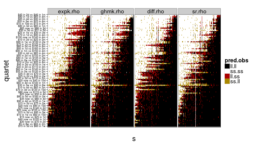
test.set.consistency(good.s)$plot
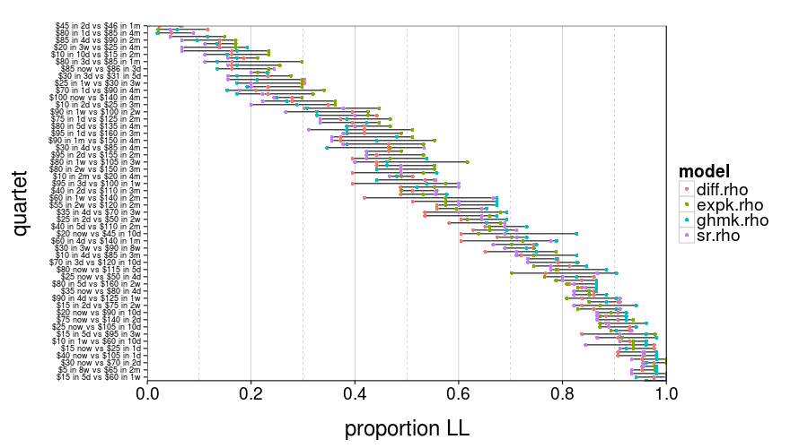
In this figure, you can see for each quartet and model group the proportion of subjects who picked LL. Those ranges look pretty wide, don't they?
round(test.set.consistency(good.s)$quantiles, 3)
| value | |
|---|---|
| 2.5% | 0.037 |
| 50% | 0.104 |
| 97.5% | 0.211 |
So the median of these ranges is 10%. That's not great.
Parameter restriction
s0175 may've suffered from the lower bound of diff.rho's prior for dr being too high. On the other hand, of the tight posteriors for dr, none go below -.4, suggesting that intervals that hit -.8 or so are just underconstrained.
sr.rho seems to have a more substantial problem with the priors being too restricted. Look at show.param(l$sr.rho, "dr") and show.param(l$sr.rho, "rho"). But let's take a closer look at the subjects whose dr s seem cut off above.
- s0040 and s0112 chose LL for every training trial, including $100 now vs. $105 in 4 months, so they were (almost?) more patient than we could've measured.
- s0104 made some weird combinations of choices in the training trials, such as LL for $100 today vs. $110 in 4 months followed by SS for $90 today vs. $95 in 4 months.
s0029 didn't seem to do anything weird, and judging from
qplot(model.sr.rho$sample.posterior(ss(ts, s == "s0029" & type == "train"), 3e5)[,"rho"], geom = "density")
his rho parameter badly wants to be higher.
I've tried widening the priors of sr.rho (I computed gamma as (1 / (1000 * rho)) instead of (1 / (100 * rho)), and tau as (exp(100 * dr) * gamma) instead of (exp(100 * dr) * gamma)) and running fit.all again. Surprisingly, although this did indeed solve the problem of, e.g., the posterior of rho for s0029 butting up against the end, prediction in the test set was generally worse than before. So so much for that.
Comparing train-to-test fits with test-to-test fits
The goal of this study has been to fit several models with a training procedure that's as ideal as possible, then use the fits thus obtained to predict performance in a separate, model-neutral test set. Perhaps we can illustrate the strengths of this approach by comparing the conclusions we get this way to conclusions we'd get from just fitting all the models directly to the test set, which is much more like the usual practice in psychology and behavioral economics. For ease of implementation, at least to begin with, let's do this test-to-test procedure the Bayesian way (albeit, again, fitting subjects indpendently, without hierarchal models) rather than using a more common technique like MLE.
fitall.train2test = cached(fit.all.train2test(good.s))
fitall.test2test = cached(fit.all.test2test(good.s))
(When I last ran the above, on 15 Jul 2013, there was only one bailout, for s0237 in train2test, who was assigned ghmk.rho.)
First, here's the mean number of correct predictions in the test set for the usual (train-to-test) procedure. The way to interpret these tables is that each row gives you the bootstrap confidence that the mean of m1 is greater than the mean of m2.
boot.correctness(fitall.train2test)
| m1 | m1.mean | m2 | m2.mean | confidence | |
|---|---|---|---|---|---|
| 1 | expk.rho | 0.859 | ghmk.rho | 0.840 | 0.88 |
| 2 | ghmk.rho | 0.840 | sr.rho | 0.809 | 0.96 |
| 3 | sr.rho | 0.809 | diff.rho | 0.742 | 1.00 |
So sr.rho made more correct predictions than diff.rho, the discounting models made more correct predictions than sr.rho and diff.rho, and ghmk.rho didn't make more correct predictions than expk.rho.
boot.correctness(fitall.test2test)
| m1 | m1.mean | m2 | m2.mean | confidence | |
|---|---|---|---|---|---|
| 1 | ghmk.rho | 0.868 | sr.rho | 0.861 | 0.80 |
| 2 | sr.rho | 0.861 | expk.rho | 0.858 | 0.68 |
| 3 | expk.rho | 0.858 | diff.rho | 0.855 | 0.63 |
Compared to the train-to-test procedure, the means are more homogeneous (confidences for the ranking are lower). Generally, they've increased, but some increases have been more dramatic.
do.call(rbind, lapply.names(models.by.name, function (m)
   {train2test = fitall.train2test[[m]]$total
    test2test = fitall.test2test[[m]]$total
    data.frame(train2test, test2test,
        diff = test2test - train2test)}))
| train2test | test2test | diff | |
|---|---|---|---|
| expk.rho | 0.859 | 0.858 | -0.001 |
| ghmk.rho | 0.840 | 0.868 | 0.028 |
| diff.rho | 0.742 | 0.855 | 0.113 |
| sr.rho | 0.809 | 0.861 | 0.052 |
Notice how the better each model did in the train-to-test procedure, the smaller the improvement in its performance by letting it peek at the test set. This is nice. It shows how the train-to-test procedure, by protecting against overfitting, did a better job than the test-to-test procedure of distinguishing among the models. It also implies that expk.rho is less readily overfit than the other models.
Now let's look at the RMSE of all the predictions. For each prediction, we calculate the error as p - t, where p is the predicted probability of choosing the larger-later option (LL), and t is 1 if the the actual choice was LL and 0 if it was SS.
boot.rmse(fitall.train2test)
| m1 | m1.mean | m2 | m2.mean | confidence | |
|---|---|---|---|---|---|
| 1 | diff.rho | 0.420 | sr.rho | 0.369 | 0.99 |
| 2 | sr.rho | 0.369 | ghmk.rho | 0.331 | 0.99 |
| 3 | ghmk.rho | 0.331 | expk.rho | 0.329 | 0.55 |
This is essentially the same ranking as for the correctness scores (except it's backwards because smaller means are better this time). Hooray, consistency.
boot.rmse(fitall.test2test)
| m1 | m1.mean | m2 | m2.mean | confidence | |
|---|---|---|---|---|---|
| 1 | diff.rho | 0.312 | expk.rho | 0.308 | 0.66 |
| 2 | expk.rho | 0.308 | sr.rho | 0.299 | 0.86 |
| 3 | sr.rho | 0.299 | ghmk.rho | 0.295 | 0.67 |
Likewise, this ranking is consistent with the one for test-to-test correctness scores.
tmm.rmse = function (tmm)
    mean(daply(ss(tmm, !is.na(trial)), .(factor(s)), function(slice)
        sqrt(mean((slice$mean - (slice$actual == "ll"))^2))))

do.call(rbind, lapply.names(models.by.name, function (m)
   {train2test = tmm.rmse(fitall.train2test[[m]]$tmm)
    test2test = tmm.rmse(fitall.test2test[[m]]$tmm)
    data.frame(
        train2test = round(train2test, 3),
        test2test = round(test2test, 3),
        diff = round(test2test - train2test, 3))}))
| train2test | test2test | diff | |
|---|---|---|---|
| expk.rho | 0.329 | 0.308 | -0.021 |
| ghmk.rho | 0.331 | 0.295 | -0.036 |
| diff.rho | 0.420 | 0.312 | -0.108 |
| sr.rho | 0.369 | 0.299 | -0.070 |
We have largely the same pattern of differences as for correctness rates.
Here are plots of the v30 parameter for expk.rho with the test-to-test procedure and train-to-test procedure. It looks like the 95% credible intervals are generally narrower for train-to-test, perhaps because of the adaptive procedure.
tmm.param.plot(fitall.train2test$expk.rho$tmm, "v30")
tmm.param.plot(fitall.test2test$expk.rho$tmm, "v30")
And now for some nigh-illegible plots of every prediction.
show.all.predictions(fitall.train2test)
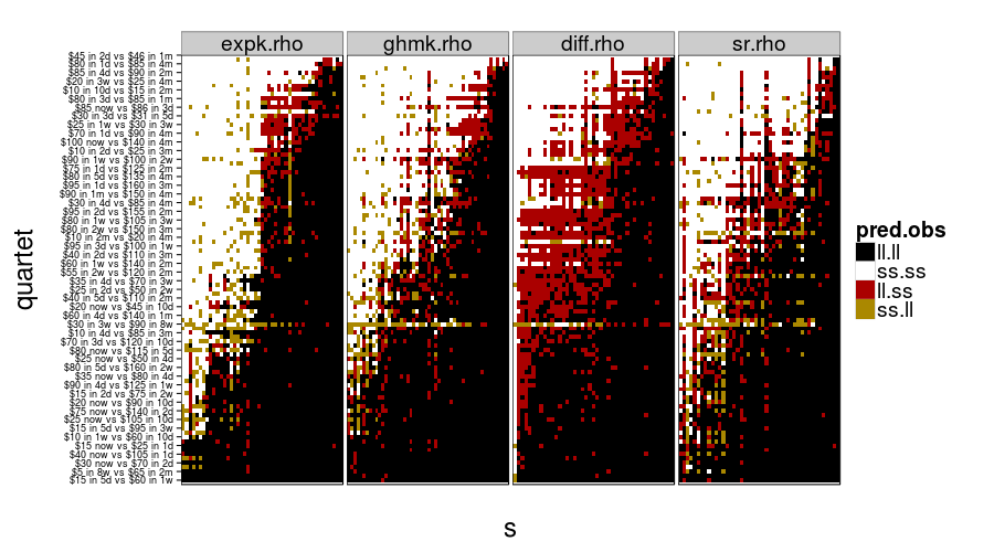
show.all.predictions(fitall.test2test)
The models look more different from each other under train-to-test, as expected. By the way, it looks like Christian was right about people not having a good sense of what 8 weeks is like, judging from the yellow horizontal stripe in every panel.
Comparing parameter estimates for expk.rho and ghmk.rho
For the exponential model and the GHM, let's see how parameter estimates differed between test-to-test and train-to-test. In these figures, for legibility, only the 95% credible intervals are shown.
ttvtt = function(model, param)
    tmms.param.plot(param.name = param, rbind(
        transform(fitall.train2test[[model]]$tmm,
            group = "train2test"),
        transform(fitall.test2test[[model]]$tmm,
            group = "test2test")))
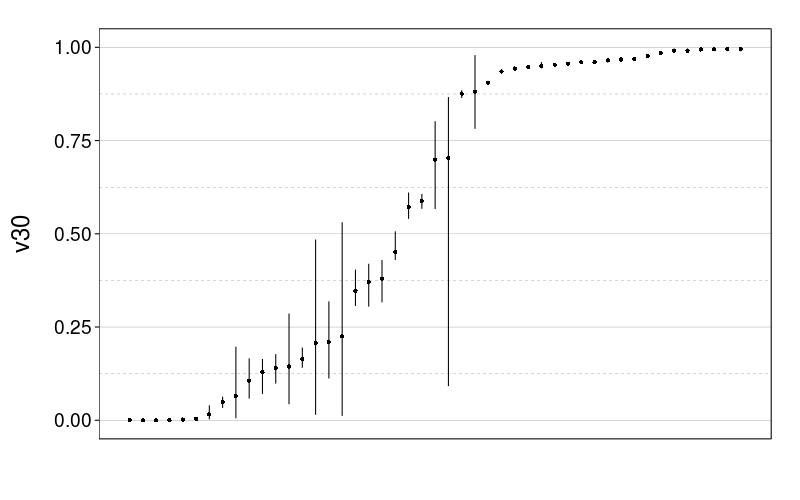
ttvtt("expk.rho", "v30") +
    scale_y_continuous(limits = c(0, 1), expand = c(0, 0))
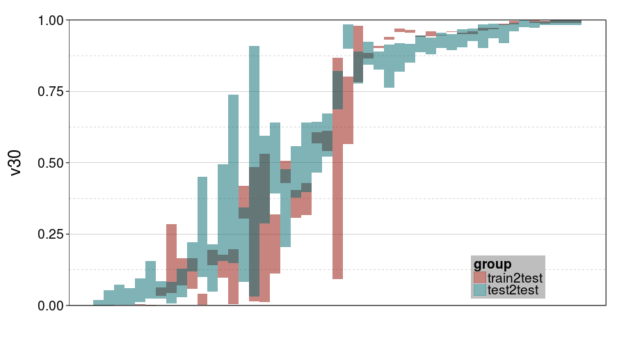
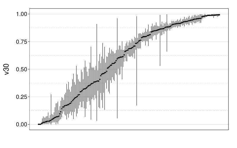
ttvtt("ghmk.rho", "v30") +
    scale_y_continuous(limits = c(0, 1), expand = c(0, 0))
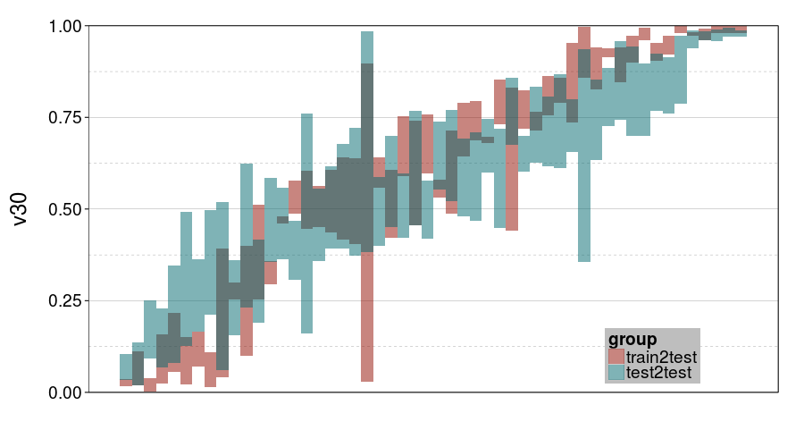
For v30, it looks like train-to-test produced tighter intervals than test-to-test. But the intervals for ghmk are wider than the intervals for expk. Also, it looks like the distribution of v30s is more bimodal for expk than ghmk.
ttvtt("expk.rho", "rho") + scale_rho
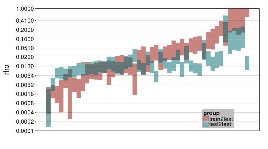
ttvtt("ghmk.rho", "rho") + scale_rho
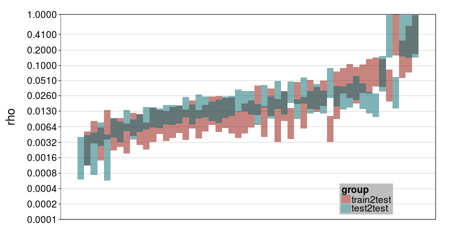
For rho, it looks like train-to-test predicted much larger individual differences than test-to-test, and this effect is greater for expk than ghmk. Perhaps as a result, there's greater agreement between the procedures for ghmk.
So one general impression I'm getting is that expk is more variable between subjects than ghmk. I guess that's a weak argument that expk is better, if we take for granted that individual differences in temporal discounting are large.
Lastly, for laughs, here's a plot for ghmk's curvature parameter.
ttvtt("ghmk.rho", "scurve") + scale_rho
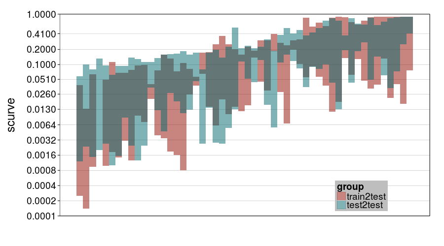
Here I guess the chief thing to observe is that there was a lot of uncertainty about curvature, with perhaps a bit more for train-to-test. Notice that most intervals contain .1 (hyperbolic discounting) and a number less than .13 (0 is exponential discounting).
Parameter correlations
Reading Peters, Miedl, and Büchel (2012) gave me the idea of checking correlations between parameters. Let's look at the between-subject correlations of posterior means. We'll use Spearman correlations to avoid scale issues.
round(digits = 3,
    tmm.param.means.cor(fitall.train2test$expk.rho$tmm))
| value | |
|---|---|
| 0.646 |
So more patient people were noisier. That's an annoyingly strong correlation, actually.
round(digits = 3,
    tmm.param.means.cor(fitall.train2test$ghmk.rho$tmm))
| scurve | rho | |
|---|---|---|
| v30 | 0.752 | 0.509 |
| scurve | 0.235 |
The correlation of v30 and rho is still here, if somewhat lesser. The correlation of v30 and scurve is substantial: more patient people had flatter discount functions.
Test-to-test AIC
aic.test2test = cached(aics.by.model(
    ss(ts, s %in% good.s & type == "test"),
    fitall.test2test))
round(digits = 2,
    boot.ranks(aic, model, data = aic.test2test, n = 5e4))
| sr.rho | expk.rho | diff.rho | |
|---|---|---|---|
| ghmk.rho | 0.61 | 0.77 | 0.95 |
| sr.rho | 0.68 | 0.91 | |
| expk.rho | 0.82 |
Paper thinking
Potential paper outline
- Introduce the idea of intertemporal choice
- Discuss past controversies on what models are appropriate
- The normative appeal of the exponential model
- The apparent descriptive superiority of a hyperbolic model (but see Luhmann (2013))
- The GHM and the two-parameter models examined in Peters et al. (2012)
- Scholten and Read's (2010) non-discounting proposal
- Argue that past head-to-head comparisons of models are limited by:
- Titration or matching procedures in preference to shuffled choices
- Test-set deficiencies
- Small size
- Ignoring front-end delays
- Using a very limited assortment of durations (e.g., just 15 days and 30 days)
- Using weird durations that people don't have a feel for (e.g., 17 days)
- Training-set deficiencies: a given set of training data may be more helpful for one model than another
- The danger of overfitting that arises from training and testing with the same data
- No explicit modeling of noise
- Using point estimates of parameters rather than marginalizing over all uncertainty in Bayesian fashion
- Introduce the four specific models tested in this study
- Present results of the test-to-test procedure (after explaining just enough of the study design so that this can be understood)
- Present results of the train-to-test procedure (after explaining the rest of the study design), contrasting them with the test-to-test results
- Toubia, Johnson, Evgeniou, and Delquié (2013)
External validity of intertemporal choice measures
- "Sketch": McKerchar and Renda (2012)
- Madden, Petry, Badger, and Bickel (1997): Heroin addicts are less patient than controls
- Sutter, Kochaer, Rützler, and Trautmann (2010): In children, impatience predicts greater spending on alcohol and cigarettes, greater BMI, and less saving
- Weller, Cook, Avsar, and Cox (2008): Obese women (but not obese men) were less patient than healthy-weight people of the same sex
- Chabris, Laibson, Morris, Schuldt, and Taubinsky (2008): Impatience predicts less frequent exercise, more smoking, and less frequently paying one's credit-card bills in full
- Khurana et al. (2012): In kids ages 10–13, impatience predicts lower likelihood of coital virginity
- Shamosh and Gray (2008): A meta-analysis concluding that intelligence is positively related to patience
- Burks, Carpenter, Goette, and Rustichini (2009): In trainee truckers, intelligence (measured by Raven's Matrices and other tests) predicts greater patience
- Demurie, Roeyers, Baeyens, and Sonuga‐Barke (2012): Kids with ADHD were less patient than autistics and controls
- Meier and Sprenger (2010): Impatience predicts greater likelihood of having credit-card debt and (conditional on having any debt) greater debt. (Debt was determined with credit reports.)
Completeness vs. accuracy
What we'd really like is a complete model of intertemporal choice. That's why observation of anomalies motivates switching to weirder models. But we can't get a complete model soon. Such a model would need to incorporate essentially everything that can influence a judgment or decision, and practically anything can:
- Some particular amounts or delays might have special meaning to some people
- If you're paid biweekly, you might compare a 2-week (but not 1-week or 3-week) reward to your paycheck
- Perhaps you need $110 for a bill
- Perhaps you think 40 is a lucky number
- Choices in one trial can be influenced by choices in past trials
- Someone might take an option because it's similar to options they took before
- Someone might apply a deliberate rule (e.g., regarding pay rate).
- Display format can influence choices
- $1 versus 100 cents
- 7 days versus 1 week
- Left side versus right side
- Non-fluent options may be rounded in different ways by different subjects
- Someone might take an option because it's easy to conceive of (fluency)
- Physiological state or other apparent influences on patience (e.g., intelligence)
- We might hope that the effect of these things can be described with the same parameters useful for describing individual differences, but that's not guaranteed.
Since completeness is out of reach, at least for the foreseeable future, it seems reasonable to ask, rather than which model is most complete, which model is most accurate overall. That is, which model can actually do the best job of predicting people's choices?
(Besides, what's the point of a complete but inaccurate model?)
A good answer to this question could be of great practical value. If there's any real connection between what intertemporal-choice tasks measure and the real-life DVs mentioned earlier, models that do a better job of predicting lab behavior should also do a better job of predicting real-life DVs.
So I set out to do a model-comparison study. There have been a lot of such studies, but mine differs because of the focus on predictive accuracy. (Also, the model set is unusually diverse.)
Within-subject consistency
Reviewer 2 for the first submission to JBDM suggested "including the same binary choices twice, and checking for consistency". The test set, by construction, had no duplicates, but we can look for duplicates in the training sets.
dodge(factor(model), unique.train, data = sb[good.s,]) + boxp +
    coord_cartesian(ylim = c(10, 50))
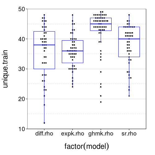
It appears that duplicates are actually very common. In fact, nobody saw 50 unique trials. Let's see how often people chose consistently across duplicates.
dupes = ddply(ss(ts, s %in% good.s),
    .(s, q = paste(ssr, ssd, llr, lld)),
    function(slice)
        if (nrow(slice) == 1)
            NULL
        else
            c(n = nrow(slice), chose.ll = sum(slice$choice == "ll")))
Note that dupes, unlike the plot above, includes the test set as well; although the test set doesn't contain any duplicates internally, the training and test sets may share quartets.
table(dupes$n)
| count | |
|---|---|
| 2 | 1041 |
| 3 | 303 |
| 4 | 138 |
| 5 | 44 |
We see that most duplicates appeared twice or thrice, although a significant minority appeared four or five times. (We're treating the same quartet as different when different subjects saw it.)
round(digits = 3, c(
    "all" = mean(with(dupes, (chose.ll/n) %in% c(0, 1))),
    "2 or 3 reps" = mean(with(ss(dupes, n %in% c(2, 3)), (chose.ll/n) %in% c(0, 1))),
    "2 reps only" = mean(with(ss(dupes, n == 2), (chose.ll/n) %in% c(0, 1)))))
| value | |
|---|---|
| all | 0.676 |
| 2 or 3 reps | 0.673 |
| 2 reps only | 0.695 |
These are the proportion of quartets for which people were perfectly consistent. I would characterize these figures as… unimpressive. To get a sense of how unimpressive, we can try something like a significance test.
round(digits = 3,
    qbinom(.999999, size = nrow(ss(dupes, n == 2)), prob = .5)/nrow(ss(dupes, n == 2)))
| value | |
|---|---|
| 0.573 |
Okay, given that that's the .999999 quantile of the relevant distribution, a boneheaded model of null responding is not, in fact, tenable. That's comforting, at least.
Now, reviewer 2 was (rightly) particularly concerned about differental random responding, or effects of random responding, between the model conditions: "If the procedure introduces more random or heuristic responding into the dataset, how this would affect the relative predictive accuracy of the models under consideration?" Let's first see how consistency compares between the model conditions.
round(digits = 3, daply(dupes,
    .(model = factor(sb[char(s), "model"])),
    function(slice)
       mean((slice$chose.ll/slice$n) %in% c(0, 1))))
| value | |
|---|---|
| diff.rho | 0.727 |
| expk.rho | 0.688 |
| ghmk.rho | 0.664 |
| sr.rho | 0.619 |
That's not great. I hoped all the figures would be about the same. I guess we have to acknowledge that it is possible the adaptive procedure induces different degrees of response noise for different models.
Test set-only validation
Reviewer 1 for JBDM wanted an analysis using half of the test set as training data and the other half as test data, and also for us to include a hyperbolic model. We can improve on this proposal by randomly splitting the data into training and test sets separately per subject.
fitall.holdout = cached(fit.all.holdout(good.s,
    holdout.factor = 1/2,
    models = c(models.by.name, list(hypk.rho = model.hypk.rho))))
dodge(Var2, value, data = melt(sapply(c(names(models.by.name), "hypk.rho"), function(m) fitall.holdout[[m]]$each.s$correct)), discrete = T) + boxp
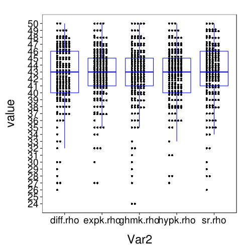
rx = simplify2array(lapply.names(fitall.holdout, function(m) daply(ss(fitall.holdout[[m]]$tmm, !is.na(trial)), .(factor(s)), function(slice) with(slice, sqrt(mean( (mean - (actual == "ll"))^2 ))))))
dodge(Var2, value, data = melt(rx)) + boxp
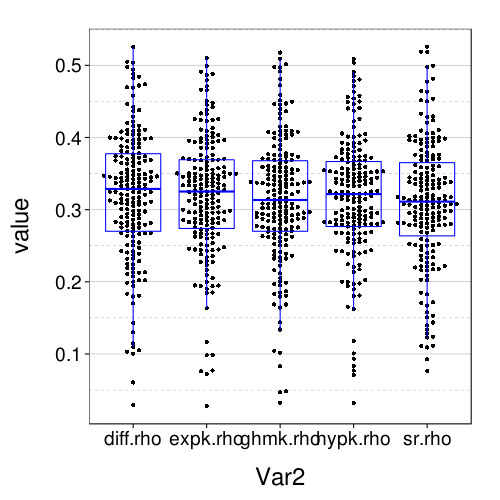
The correct-count and RMSE ratings shown here are for all models similar to the performance of Exp under train-to-test. So it seems that the effect of using the adaptive procedure for training, rather than more trials of the kind that appear the test set, is only to worsen the performance of Diff and SR, and with this obstacle removed, all the models perform about the same.
Oops?
Cross-validation
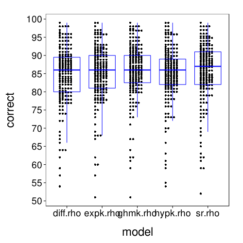
Now let's try 5-fold cross-validation within the test set.
fitall.xvalid = cached(fit.all.xvalid(
    good.s,
    folds = 5,
    models = c(models.by.name, list(hypk.rho = model.hypk.rho)),
    ts))

fitall.xvalid.correct = ss(
    melt(sapply(c(names(models.by.name), "hypk.rho"),
        function(m) with(fitall.xvalid[[m]], tapply((mean >= .5) == (actual == "ll"), s, sum)))),
    !is.na(value))
names(fitall.xvalid.correct) = qw(s, model, correct)
dodge(model, correct, discrete = T, data = fitall.xvalid.correct) +
    scale_y_continuous(breaks = seq(50, 100, 5)) +
    boxp
rx = simplify2array(lapply.names(fitall.xvalid,
    function(m) daply(fitall.xvalid[[m]], .(factor(s)), function(slice)
        with(slice, sqrt(mean( (mean - (actual == "ll"))^2 ))))))
dodge(Var2, value, data = melt(rx)) + boxp
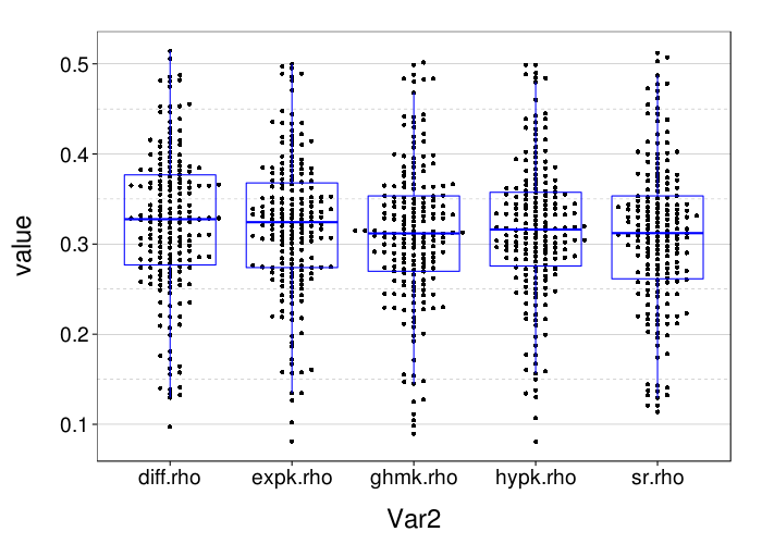
These results for correct-count and RMSE look very similar to the results for one-round validation presented previously.
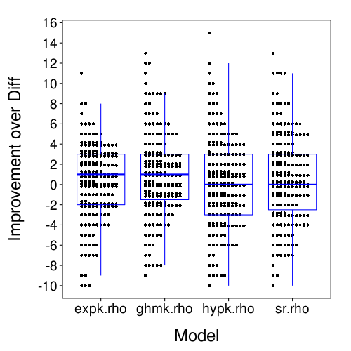
How about within-subjects comparisons of these cross-validations?
x = ss(
    data.frame(sapply(c(names(models.by.name), "hypk.rho"),
        function(m) with(fitall.xvalid[[m]],
            tapply((mean >= .5) == (actual == "ll"), s, sum)))),
    !is.na(expk.rho))
dodge(Var2, value, discrete = T, stack.width = 10,
    data = melt(ss(t(maprows(x, function(v) v - v["diff.rho"])),
        select = -diff.rho))) +
    boxp +
    scale_y_continuous(name = "Improvement over Diff",
        breaks = seq(-10, 16, 2)) +
    xlab("Model")
x = simplify2array(lapply.names(fitall.xvalid,
    function(m) daply(fitall.xvalid[[m]], .(factor(s)), function(slice)
        with(slice, sqrt(mean( (mean - (actual == "ll"))^2 ))))))
dodge(Var2, value,
    data = melt(ss(t(maprows(x, function(v) v["diff.rho"] - v)),
        select = -diff.rho))) +
    boxp +
    scale_y_continuous(name = "Improvement over Diff") +
    xlab("Model")
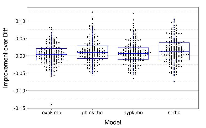
Here is a table of for each model, the number of subjects whose lowest RMSE was for that model.
sort(table(maprows(x, function(v) names(v)[which.min(v)])), dec = T)
| value | |
|---|---|
| sr.rho | 70 |
| diff.rho | 42 |
| expk.rho | 28 |
| hypk.rho | 24 |
| ghmk.rho | 23 |
sr.rho (BT) is the clear winner by this metric. But here is a measure of within-subject variability of RMSE: the quantiles of the ranges of RMSE between the five models.
round(d = 3, quantile(
    maprows(x, function(v) max(v) - min(v)),
    c(.025, .25, .5, .75, .975)))
| value | |
|---|---|
| 2.5% | 0.008 |
| 25% | 0.022 |
| 50% | 0.038 |
| 75% | 0.055 |
| 97.5% | 0.105 |
This seems to imply that within-subject differences in model accuracy are generally small.
Other learners
Rationale
We now seem to be in the surprising situation where all the models are performing about the same, with accuracy around 86% and RMSE around .325.
There are all sorts of things we could look at in order to try to explain why all the models are performing similarly to each other and why cross-validated test error is hardly more than the training error. But we have little ability to distinguish plausible explanations from correct explanations without collecting new data for the purpose. Which is one of the problems with explanatory science, of course.
Let's instead back up a bit and frame the question of this project (and the eventual paper) as "What sorts of predictive procedures are good in this situation?", where "this situation" is now prediction of the test set with (disjoint pieces of) itself. We'll investigate a few other predictive procedures, including very simple things like the majority model (analyzed predictively, not prophetically as in the first manuscript) and perhaps naive Bayes, and also heavier-duty machine-learning techniques like decision trees. Non-Bayesian applications of the existing models would also make sense. The goal is to identify what is the best predictive accuracy achievable (and with which procedures) and what is the simplest procedure one can use that still achieves respectable accuracy. We might also try changing the training-set size to see how it affects these matters.
SVM tuning
svm.explore = function(gamma, cost)
    do.call(rbind, lapply(good.s, function(the.s) {message(the.s); t = ss(ts, char(s) == the.s & type == "test"); if (any(table(t$choice) < 4)) return(NULL); iv = t[qw(ssr, ssd, llr, lld)]; for (col in seq_len(ncol(iv))) iv[,col] = zscore(iv[,col]); data.frame(s = the.s, tune.svm(x = iv, y = t$choice, scale = F, type = "C-classification", cost = cost, gamma = gamma)$performances[qw(gamma, cost, error)])}))

# svm.optim = function(the.s)
#    {message(the.s);
#     t = ss(ts, char(s) == the.s & type == "test");
#     if (any(table(t$choice) < 4))
#         return(NULL);
#     iv = t[qw(ssr, ssd, llr, lld)];
#     for (col in seq_len(ncol(iv))) iv[,col] = zscore(iv[,col])
#     dv = t$choice
#     o = optim(c(-13, 19),
#         fn = function(p)
#             tune.svm(x = iv, y = dv,
#                 scale = F, type = "C-classification",
#                 gamma = 2^p[1], cost = 2^p[2])$best.performance,
# #        method = "BFGS",
#         control = list(trace = 1, maxit = 25, reltol = 1e-2))
#     o}

svm.perfs = rbind(
    cached(do.call(rbind, lapply(good.s, function(the.s) {message(the.s); t = ss(ts, char(s) == the.s & type == "test"); if (any(table(t$choice) < 4)) return(NULL); iv = t[qw(ssr, ssd, llr, lld)]; for (col in seq_len(ncol(iv))) iv[,col] = zscore(iv[,col]); data.frame(s = the.s, tune.svm(x = iv, y = t$choice, scale = F, type = "C-classification", cost = 2^seq(-5, 15, 2), gamma = 2^seq(-15, 3, 2))$performances[qw(gamma, cost, error)])}))),
    cached(do.call(rbind, lapply(good.s, function(the.s) {message(the.s); t = ss(ts, char(s) == the.s & type == "test"); if (any(table(t$choice) < 4)) return(NULL); iv = t[qw(ssr, ssd, llr, lld)]; for (col in seq_len(ncol(iv))) iv[,col] = zscore(iv[,col]); data.frame(s = the.s, tune.svm(x = iv, y = t$choice, scale = F, type = "C-classification", cost = 2^seq(17, 21, 2), gamma = 2^seq(-15, 5, 2))$performances[qw(gamma, cost, error)])}))),
    cached(svm.explore(gamma = 2^c(-17, -19, -21), cost = 2^c(23, 25, 27))),
    cached(svm.explore(gamma = 2^c(-17, -19, -21), cost = 2^c(17, 19, 21))),
    cached(svm.explore(gamma = 2^c(-15, -13, -11), cost = 2^c(23, 25, 27))))
svm.perfs = transform(svm.perfs, gamma = log(gamma, 2), cost = log(cost, 2))
ggplot(aggregate(excess ~ gamma + cost,
       ddply(svm.perfs, .(s), function(slice) transform(slice, excess = error - min(error))),
       function (v) sum(v^2))) +
    geom_raster(aes(gamma, cost, fill = excess)) +
    scale_fill_gradient(low = "gray80", high = "black") +
    geom_text(aes(gamma, cost, label = round(100*excess))) +
    geom_point(aes(x, y), data = expand.grid(x = seq(-25, 5, len = 5), y = seq(-5, 25, len = 5)), color = "blue")
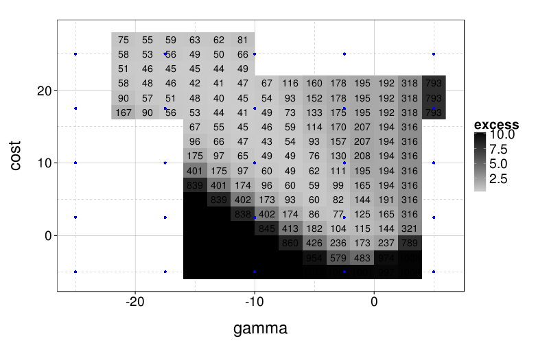
I don't really want to "overfit" my SVM tuning to the results here, not least because the surface could look quite different when there's lots of noise or the training set is small. And I guess I want to stick to a grid search, because that's standard practice, and designing an effective yet fast method of adaptively tuning SVM hyperparameters is probably not worth my time for this project. So I'll do a grid search on the blue points.
Comparison of robustness
We will repeat the cross-validation analyses from before, except that in each fold, we'll randomly tamper with a fixed portion of the training set. For the choice we want to corrupt, we'll choose at random whether to replace it with SS or LL rather than always changing it to its reverse (which I suspect is too harsh to more complex models).
correct.by.integrity = cached(metaparam.xvalid(
    corrupt.training.data.mxw,
    good.s,
    c(90, 70, 60, 50, 30, 15, 10)))
correct.by.train.size.plot(T, aggregate(
        correct ~ learner + train.size,
        correct.by.integrity,
        median)) +
    coord_cartesian(xlim = c(10, 90), ylim = c(50, 90)) +
    xlab("Uncorrupted training trials") +
    ylab("Median correct predictions")

Here diff.glm seems to be the clear winner. Although its performance deteriorates as the training set is corrupted, it tends to do much better than other models facing the same amount of noise.
correct.by.train.size.plot(T, aggregate(
        correct ~ learner + train.size,
        correct.by.integrity,
        function (v) quantile(v, .1))) +
    coord_cartesian(xlim = c(10, 90), ylim = c(40, 80)) +
    xlab("Uncorrupted training trials") +
    ylab("First decile of correct predictions")
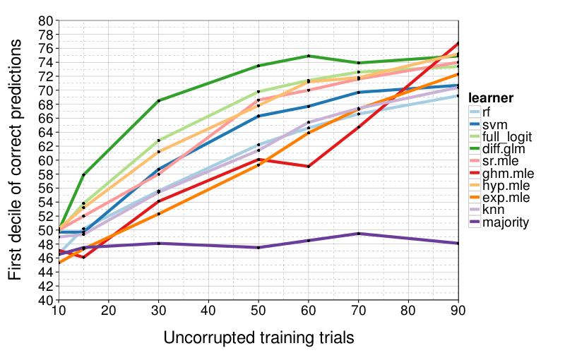
diff.glm isn't as consistently good when we look at worse cases, the first decile of performance. Here there's a less clear winner, although sr.mle and hyp.mle are good across-the-board performers, and diff.glm only gets bad when train.size = 5.
Comparison of training-set sizes
correct.by.train.size = cached(metaparam.xvalid(
    shrink.training.data.mxw,
    good.s,
    c(90, 70, 60, 50, 30, 15, 10)))
correct.by.train.size.plot(T, aggregate(
        correct ~ learner + train.size,
        correct.by.train.size,
        median)) +
    coord_cartesian(xlim = c(10, 90), ylim = c(50, 90)) +
    ylab("Median correct predictions")
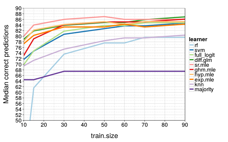
sr.mle is slightly better than diff.glm and hyp.mle, which are about evenly matched.
correct.by.train.size.plot(T, aggregate(
        correct ~ learner + train.size,
        correct.by.train.size,
        function (v) quantile(v, .1))) +
    coord_cartesian(xlim = c(10, 90), ylim = c(40, 80)) +
    ylab("First decile of correct predictions")
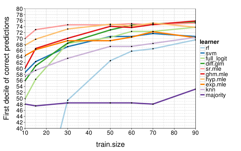
Now diff.glm isn't doing so hot. sr.mle and hyp.mle continue to do well.
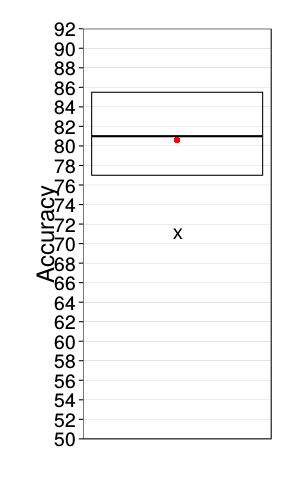
New analyses for BJDSM submission 2
Differences between MTurk and lab
dodge(ifelse(is.na(worker), "Lab", "MTurk"), test.lls, data = sb[good.s,]) +
    boxp
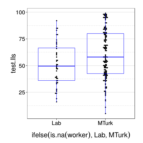
Looks like MTurk subjects are more patient.
correct.lab = cached(metaparam.xvalid(
    shrink.training.data.mxw,
    row.names(ss(sb, good & is.na(worker))),
    90))
correct.mturk = cached(metaparam.xvalid(
    shrink.training.data.mxw,
    row.names(ss(sb, good & !is.na(worker))),
    90))
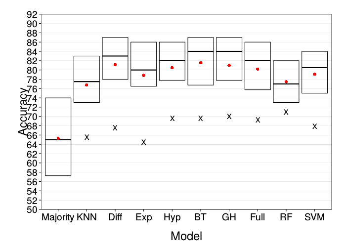
ggplot(prettify.lnames(ss(correct.lab, train.size == 90))) +
    stat_summary(aes(learner, correct), geom = "crossbar",
        fun.data = function(y)
            `names<-`(quantile(y, c(.25, .5, .75)), qw(ymin, y, ymax))) +
    stat_summary(aes(learner, correct), geom = "point",
        fun.y = function(y) quantile(y, .1),
        shape = "X", size = 5) +
    stat_summary(aes(learner, correct), geom = "point",
        fun.y = mean,
        color = "red", size = 3) +
    scale_y_continuous(breaks = seq(0, 100, 2), minor_breaks = NULL) +
    coord_cartesian(ylim = c(50, 92)) +
    xlab("Model") + ylab("Accuracy") +
    theme(
        panel.grid.major.x = element_blank(),
        panel.grid.major.y = element_line(colour = "gray50", size = 0.07))
ggplot(prettify.lnames(ss(correct.mturk, train.size == 90))) +
    stat_summary(aes(learner, correct), geom = "crossbar",
        fun.data = function(y)
            `names<-`(quantile(y, c(.25, .5, .75)), qw(ymin, y, ymax))) +
    stat_summary(aes(learner, correct), geom = "point",
        fun.y = function(y) quantile(y, .1),
        shape = "X", size = 5) +
    stat_summary(aes(learner, correct), geom = "point",
        fun.y = mean,
        color = "red", size = 3) +
    scale_y_continuous(breaks = seq(0, 100, 2), minor_breaks = NULL) +
    coord_cartesian(ylim = c(50, 92)) +
    xlab("Model") + ylab("Accuracy") +
    theme(
        panel.grid.major.x = element_blank(),
        panel.grid.major.y = element_line(colour = "gray50", size = 0.07))
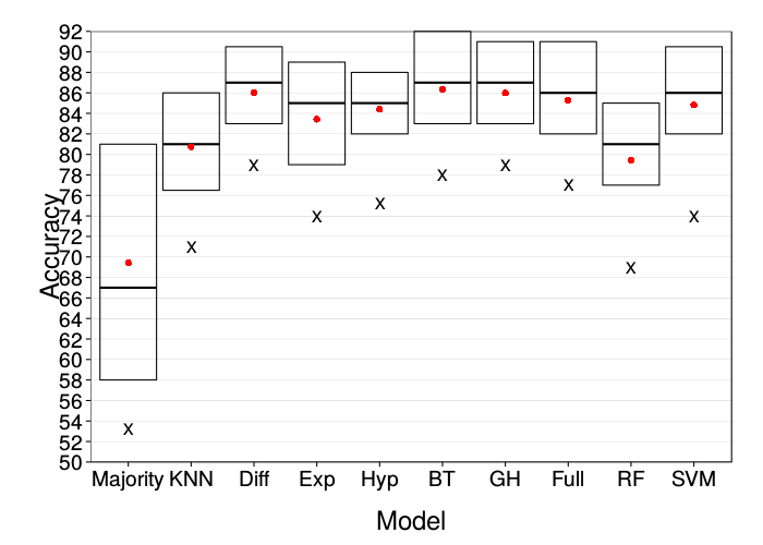
These are both comparable to the original figure.
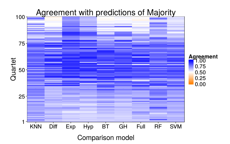
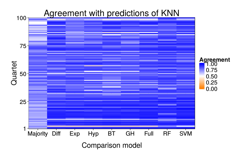
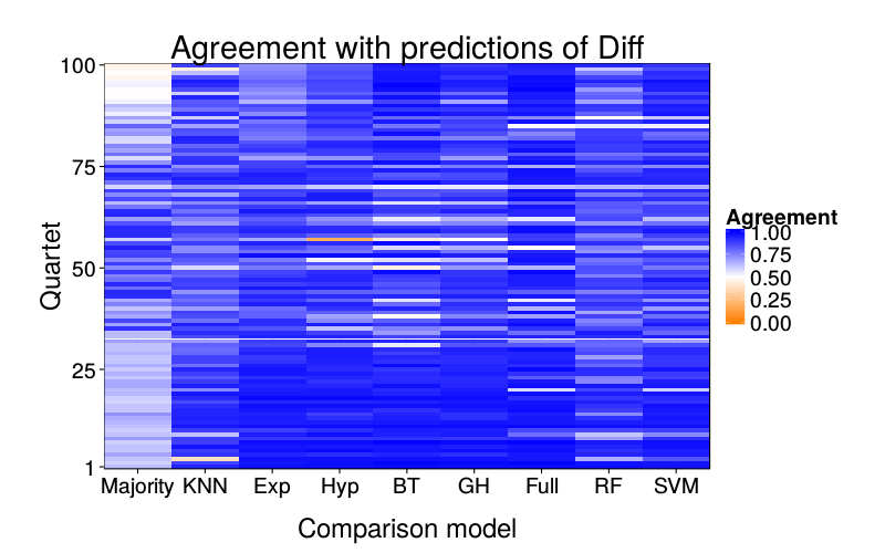
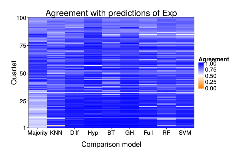
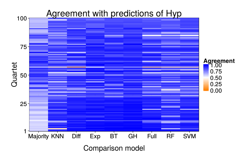
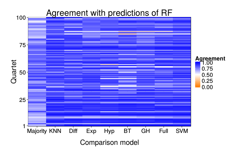
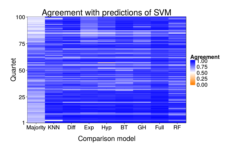
Prediction overlap
indpred = cached(ordf(individual.xvalid(good.s), learner, s, qn))
indpred$predll = indpred$pred == "ll"
indpred.ary = acast(indpred, learner ~ qn ~ s, value.var = "predll")
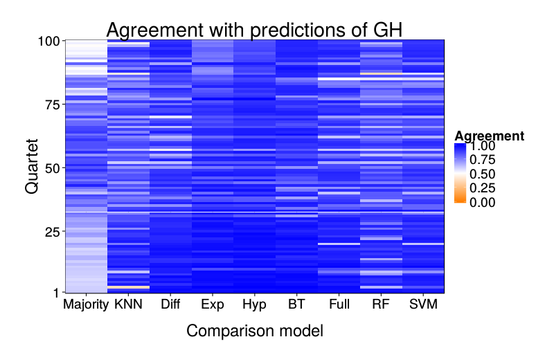
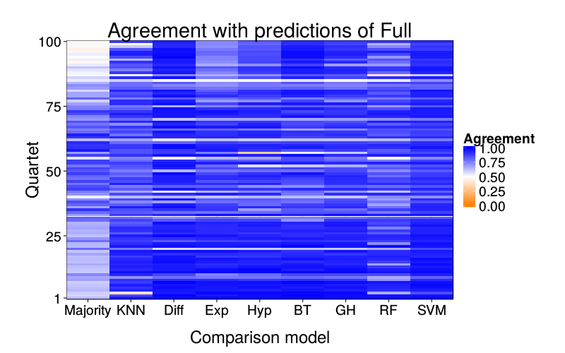
overlap.plot = function(focal.lname)
{focus = indpred.ary[focal.lname,,]
d = prettify.lnames(do.call(rbind, lapply(setdiff(names(learners), focal.lname), function(comparison.lname)
data.frame(
learner = comparison.lname,
qn = 1 : nrow(focus),
agree = rowMeans(focus == indpred.ary[comparison.lname,,])))))
ggplot(d) +
ggtitle(paste("Agreement with predictions of",
names(pretty.learner.names)[pretty.learner.names == focal.lname])) +
geom_tile(aes(learner, qn, fill = agree)) +
scale_fill_gradient2(name = "Agreement",
limits = c(0, 1), midpoint = .5,
low = "#ff7f00", high = "blue") +
scale_y_continuous(name = "Quartet", expand = c(0, 0), breaks = c(1, 25, 50, 75, 100)) +
scale_x_discrete(name = "Comparison model", expand = c(0, 0))}
overlap.plot("majority")
overlap.plot("knn")
overlap.plot("diff.glm")
overlap.plot("exp.mle")
overlap.plot("hyp.mle")
overlap.plot("sr.mle")
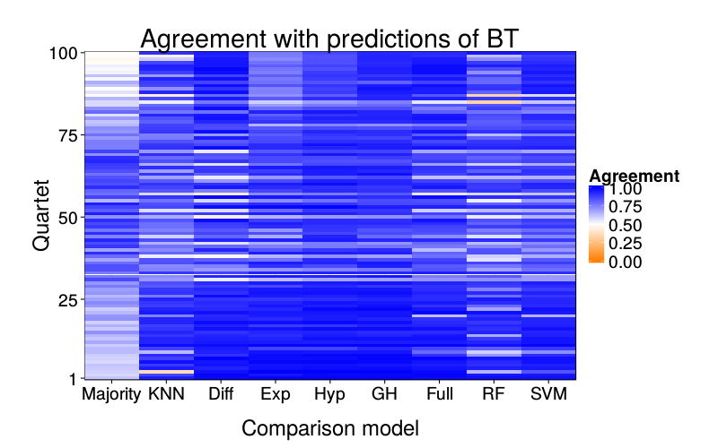
overlap.plot("ghm.mle")
overlap.plot("full_logit")
overlap.plot("rf")
overlap.plot("svm")
Saturated logit model
xvalid.saturated = cached(individual.xvalid(good.s,
    lnames = "saturated_logit",
    extra.learners = list(saturated_logit = extra.learner.saturated_logit)))
ggplot(data.frame(correct = daply(xvalid.saturated, .(factor(s)),
        function(x) sum(x$choice == x$pred)))) +
    stat_summary(aes(1, y = correct), geom = "crossbar",
        fun.data = function(y)
            `names<-`(quantile(y, c(.25, .5, .75)), qw(ymin, y, ymax))) +
    stat_summary(aes(1, y = correct), geom = "point",
        fun.y = function(y) quantile(y, .1),
        shape = "X", size = 5) +
    stat_summary(aes(1, y = correct), geom = "point",
        fun.y = mean,
        color = "red", size = 3) +
    scale_y_continuous(breaks = seq(0, 100, 2), minor_breaks = NULL) +
    scale_x_continuous(name = "", breaks = c()) +
    coord_cartesian(ylim = c(50, 92)) +
    ylab("Accuracy") +
    theme(
        panel.grid.major.x = element_blank(),
        panel.grid.major.y = element_line(colour = "gray50", size = 0.07))
References
Burks, S. V., Carpenter, J. P., Goette, L., & Rustichini, A. (2009). Cognitive skills affect economic preferences, strategic behavior, and job attachment. Proceedings of the National Academy of Sciences, 106(19), 7745–7750. doi:10.1073/pnas.0812360106
Chabris, C. F., Laibson, D., Morris, C. L., Schuldt, J. P., & Taubinsky, D. (2008). Individual laboratory-measured discount rates predict field behavior. Journal of Risk and Uncertainty, 37(2, 3), 237–269. doi:10.1007/s11166-008-9053-x
Demurie, E., Roeyers, H., Baeyens, D., & Sonuga‐Barke, E. (2012). Temporal discounting of monetary rewards in children and adolescents with ADHD and autism spectrum disorders. Developmental Science, 15(6), 791–800. doi:10.1111/j.1467-7687.2012.01178.x
Khurana, A., Romer, D., Betancourt, L. M., Brodsky, N. L., Giannetta, J. M., & Hurt, H. (2012). Early adolescent sexual debut: The mediating role of working memory ability, sensation seeking, and impulsivity. Developmental Psychology, 48(5), 1416–1428. doi:10.1037/a0027491
Luhmann, C. C. (2013). Discounting of delayed rewards is not hyperbolic. Journal of Experimental Psychology: Learning, Memory, and Cognition, 39(4), 1274–1279. doi:10.1037/a0031170
Madden, G. J., Petry, N. M., Badger, G. J., & Bickel, W. K. (1997). Impulsive and self-control choices in opioid-dependent patients and non-drug-using control participants: Drug and monetary rewards. Experimental and Clinical Psychopharmacology, 5(3), 256–262. doi:10.1037/1064-1297.5.3.256
McKerchar, T. L., & Renda, C. R. (2012). Delay and probability discounting in humans: An overview. Psychological Record, 62(4), 817–834.
Meier, S., & Sprenger, C. D. (2010). Present-biased preferences and credit card borrowing. American Economic Journal: Applied Economics, 2(1), 193–210. doi:10.1257/app.2.1.193
Peters, J., Miedl, S. F., & Büchel, C. (2012). Formal comparison of dual-parameter temporal discounting models in controls and pathological gamblers. PLOS ONE. doi:10.1371/journal.pone.0047225
Scholten, M., & Read, D. (2010). The psychology of intertemporal tradeoffs. Psychological Review, 117(3), 925–944. doi:10.1037/a0019619. Retrieved from http://repositorio.ispa.pt/bitstream/10400.12/580/1/rev-117-3-925.pdf
Scholten, M., & Read, D. (2013). Time and outcome framing in intertemporal tradeoffs. Journal of Experimental Psychology: Learning, Memory, and Cognition, 39(4), 1192–1212. doi:10.1037/a0031171
Shamosh, N. A., & Gray, J. R. (2008). Delay discounting and intelligence: A meta-analysis. Intelligence, 36(4), 289–305. doi:10.1016/j.intell.2007.09.004
Sutter, M., Kochaer, M. G., Rützler, D., & Trautmann, S. T. (2010). Impatience and uncertainty: Experimental decisions predict adolescents' field behavior (Discussion Paper No. 5404). Institute for the Study of Labor. Retrieved from http://ftp.iza.org/dp5404.pdf
Toubia, O., Johnson, E., Evgeniou, T., & Delquié, P. (2013). Dynamic experiments for estimating preferences: An adaptive method of eliciting time and risk parameters. Management Science, 59(3), 613–640. doi:10.1287/mnsc.1120.1570
Weller, R. E., Cook, E. W., III, Avsar, K. B., & Cox, J. E. (2008). Obese women show greater delay discounting than healthy-weight women. Appetite, 51(3), 563–569. doi:10.1016/j.appet.2008.04.010