Comorbid notebook
Created 2 Aug 2016 • Last modified 5 Oct 2017
The context of the data
All results with cell sizes 10 or below need approval to be distributed in any manner.
Jennifer:
- "for the comorbidity analysis, we have only been using 2010 data since it's the most recent we have. The 3 analysis files (all_*) were created using the 2010 claims."
- "the three all_* files will be best for you to work with, so you don't have to deal with the raw claims quite yet. When we asked for the data, we didn't get all Medicare/Medicaid enrollees, we only got those who had an ARV claim or HIV diagnosis at any point. Then we further refine our sample using the algorithm. Due to the nature of claims, we also have to limit to people enrolled for the full year, are fee-for-service (rather than managed care), and are in California the entire year"
- "Regarding the ID variables, bene_id is the Medicare ID so we use it for Medicare only and Duals and msis_id is the Medicaid ID which we use for Medicaid only patients. Throughout the years, Medicaid patients have gradually also been assigned a bene_id, but there are still some people who don't have one. The reason we have bene_id_10 is because we found inconsistencies in IDs when merging across years, this version is needed to merge with raw claims for that year. The bene_id variable allows for consistency in merging across years.… There are a few other caveats with the ID variables we can discuss at a later point when needed."
- The three files have the same variables
Redacted claims
Jennifer: "Claims relating to substance abuse were redacted for our 2009 and 2010 data, thus these payments are not included in our individual claims. Thus, we will find lower total costs for those who have redacted claims."
| Eligibility | Claim Type | # Suppressed Claims | Total Claims | % Claims Suppressed | # Beneficiaries w/ Suppressed Claims | Total Beneficiaries in Claims | % Beneficiaries w/ Suppressed Claims | Medicaid Payment (MDCD_PYMT_AMT) Suppressed Claims | Total Medicaid Payment (MDCD_PYMT_AMT) in Claims |
|---|---|---|---|---|---|---|---|---|---|
| All | Inpatient | 773,353 | 9,378,620 | 8.25% | 417,977 | 6,106,602 | 6.84% | 3,040,765,005 | 35,166,806,936 |
| Long-Term Care | 225,235 | 33,319,656 | 0.68% | 38,945 | 1,648,083 | 2.36% | 522,839,791 | 62,508,895,726 | |
| Other Services | 37,376,167 | 2,520,159,210 | 1.48% | 1,415,671 | 62,063,859 | 2.28% | 1,706,728,920 | 213,731,343,805 | |
| Total | 38,374,755 | 2,562,857,486 | 1.50% | 1,628,983 | 62,381,748 | 2.61% | 5,270,333,716 | 311,407,046,467 | |
| Aged | Inpatient | 19,737 | 951,402 | 2.07% | 16,697 | 618,562 | 2.70% | 41,584,740 | 1,973,545,032 |
| Long-Term Care | 71,432 | 22,972,515 | 0.31% | 5,426 | 1,081,340 | 0.50% | 151,269,024 | 36,690,837,529 | |
| Other Services | 441,310 | 239,166,210 | 0.18% | 24,220 | 4,100,416 | 0.59% | 22,440,257 | 25,928,333,797 | |
| Total | 532,479 | 263,090,127 | 0.20% | 41,666 | 4,258,713 | 0.98% | 215,294,021 | 64,592,716,358 | |
| Disabled / Blind | Inpatient | 389,806 | 2,831,711 | 13.77% | 215,676 | 1,418,478 | 15.20% | 1,806,188,438 | 16,188,598,664 |
| Long-Term Care | 98,952 | 9,466,201 | 1.05% | 17,048 | 457,139 | 3.73% | 242,493,452 | 23,612,634,633 | |
| Other Services | 15,469,683 | 772,861,048 | 2.00% | 549,705 | 9,493,018 | 5.79% | 674,012,800 | 90,720,882,400 | |
| Total | 15,958,441 | 785,158,960 | 2.03% | 658,766 | 9,524,493 | 6.92% | 2,722,694,690 | 130,522,115,697 | |
| Child | Inpatient | 27,627 | 2,314,122 | 1.19% | 21,927 | 1,794,121 | 1.22% | 124,069,187 | 7,485,361,209 |
| Long-Term Care | 42,109 | 414,447 | 10.16% | 10,291 | 72,559 | 14.18% | 98,818,837 | 1,267,625,658 | |
| Other Services | 3,514,205 | 977,750,886 | 0.36% | 220,256 | 32,530,394 | 0.68% | 241,240,915 | 54,673,886,767 | |
| Total | 3,583,941 | 980,479,455 | 0.37% | 235,895 | 32,561,585 | 0.72% | 464,128,939 | 63,426,873,634 | |
| Adult | Inpatient | 303,819 | 2,941,126 | 10.33% | 144,368 | 2,052,181 | 7.03% | 908,646,835 | 8,006,862,338 |
| Long-Term Care | 8,499 | 119,370 | 7.12% | 4,976 | 20,899 | 23.81% | 15,911,261 | 131,464,388 | |
| Other Services | 16,739,091 | 480,568,052 | 3.48% | 586,975 | 15,494,187 | 3.79% | 730,157,393 | 37,339,227,221 | |
| Total | 17,051,409 | 483,628,548 | 3.53% | 647,872 | 15,573,669 | 4.16% | 1,654,715,489 | 45,477,553,947 |
(Only the claims that contain the substance abuse codes are removed; not the beneficiary and all claims associated with that beneficiary)
The "MAX Uniform Eligibility Code - For Month of Service" (EL_MAX_ELGBLTY_CD_MO) variable from each claim was used to determine eligibility grougs.
- Aged: 11, 21, 31, 41, 51
- Blind/Disabled: 12, 22, 32, 42, 52
- Child: 14, 16, 24, 34, 44, 48, 54
- Adult: 15, 17, 25, 35, 45, 55, 3A
Descriptives
These demographic tables use the same sample inclusion criteria as the association analyses described below.
(display-demog "mcare_only")
| I | value |
|---|---|
| Female, proportion | .048 |
| Age, minimum | 31 |
| Age, median | 56 |
| Age, maximum | 94 |
| Race, white, proportion | .761 |
| Race, black, proportion | .070 |
| Race, Hispanic, proportion | .117 |
| Race, other, proportion | .052 |
| Urban, proportion | .949 |
| High-volume HIV care provider, proportion | .582 |
| Disabled, proportion | .773 |
(display-demog "dual")
| I | value |
|---|---|
| Female, proportion | .118 |
| Age, minimum | 21 |
| Age, median | 50 |
| Age, maximum | 90 |
| Race, white, proportion | .527 |
| Race, black, proportion | .212 |
| Race, Hispanic, proportion | .223 |
| Race, other, proportion | .038 |
| Urban, proportion | .944 |
| High-volume HIV care provider, proportion | .661 |
| Disabled, proportion | .955 |
Prediction of total costs
These cross-validation analyses of predictive accuracy use all beneficiaries from 2010. The predictors are gender, race, age, age squared, disabled status, and each of the comorbid conditions.
| mcaid_only | mcare_only | dual | |
|---|---|---|---|
| Trivial (predict median) | 18,918 | 22,280 | 26,439 |
| OLS (no log transformation) | 17,819 | 21,613 | 23,801 |
| OLS | 17,455 | 22,399 | 22,470 |
| Ridge regression | 17,503 | 22,377 | 22,448 |
| Elastic net | 17,422 | 22,267 | 22,428 |
| Elastic net w/ all 1st-order interactions | 17,304 | 22,497 | 22,407 |
| Quantile regression | 17,053 | 20,279 | 22,327 |
| Quantile regression w/ lasso | 17,090 | 20,597 | 22,354 |
| Quantile regression w/ lasso, some interactions | 17,152 | 20,832 | 22,420 |
| Quantile regression w/ lasso, inpatient | 17,338 | 21,394 | 25,516 |
| Random forest | 18,940 | 23,274 | 24,231 |
| [Min MAE, gender and race] | 18,834 | 22,207 | 26,408 |
| [Min MAE, all IVs but age] | 11,594 | 12,977 | 13,811 |
Here, for each of the three datasets and several models, we have the cross-validated mean absolute error (MAE) in predicting total expenditure per subject, in dollars. This means that, e.g., a MAE of $15,000 implies that the model's point prediction of a beneficiary's expenditures would have a mean distance from the true value of $15,000.
Except where marked, each model log-transforms the DV for model-fitting, then exp-transforms the predictions. You can see that this trick increases predictive accuracy (according to MAE) quite a bit.
The best-performing model in each case is unregularized quantile regression. In the case of Medicare-only beneficiares, there is a large improvement upon OLS.
Regularization (as the lasso) is necessary for the more complex quantile regression models because the model-fitting procedure has problems finding a solution otherwise. "Quantile regression w/ lasso, some interactions" interacts age and age squared with each comorbidity, and gender with each race. "Quantile regression w/ lasso, inpatient" uses logistic regression to predict whether the patient had any inpatient costs, and then applies a separately trained quantile regression model depending on each patient's predicted inpatient status.
The last two rows give a kind of lower bound on possible MAE for the demographic IVs and all IVs (demographic variables plus comorbidity flags), respectively. They are simply the MAE achieved when each subject's true value is predicted with the median among all subjects with precisely the same IV values (except for age, since it's continuous, unlike all the other IVs). So, unless age is very informative, we can't get MAEs below these numbers, and we probably won't be able to get MAEs very near them, either; getting a MAE that low in training would almost certainly lead to overfitting in testing.
Prediction of individual cost types
Thinking
Let's log the DV, as before.
Let's compare trivial models (i.e. predicting the median and ignoring all IVs) to quantile regression. Let's also compare models that have only the demographic variables as IVs to models that have comorbidities. And, let's compare models with a dummy variable for having Medicaid to twinned models (one for Medicare only, one for duals). That means we have…
- Trivial, single
- Trivial, twinned
- Quantile regression, demographic IVs, single
- Quantile regression, demographic IVs, twinned
- Quantile regression, all IVs, single
- Quantile regression, all IVs, twinned
…for each of the three cost types, and then there's the question of how to handle the (zero-inflated) inpatient costs. All the above methods could be applied unaltered, or you could precede them with a logistic-regression model that decides whether the patient has nonzero inpatient costs, and we can imagine four ways to use this logistic-regression model based on the choice of IVs (demographic-only versus all) and how we deal with Medicare-only versus duals (dummy variable versus twinned models). Ouch! But from talking to Arleen and Jennifer, I guess we'd best bite the bullet and consider all 16 nontrivial models for inpatient costs.
Since twin models didn't prevail for outpatient or drug costs, let's forget about those. That gives us the following models for inpatient costs:
- Fully trivial: just guess the median
- Quantile regression only (demographic IVs)
- Quantile regression only (all IVs)
- Logistic regression for nonzero (demographic IVs), then guess the conditional median
- Logistic regression for nonzero (demographic IVs), then quantile regression (demographic IVs)
- Logistic regression for nonzero (demographic IVs), then quantile regression (all IVs
- Logistic regression for nonzero (all IVs), then guess the conditional median
- Logistic regression for nonzero (all IVs), then quantile regression (demographic IVs)
- Logistic regression for nonzero (all IVs), then quantile regression (all IVs)
Results
Absolute error
(display-pred-cv pred-cv-orx-mae)
| I | DV | IVs | twin | MAE |
|---|---|---|---|---|
| 0 | y_outpatient | trivial | single | 6,565 |
| 1 | y_outpatient | trivial | twin | 6,555 |
| 2 | y_outpatient | demog | single | 6,495 |
| 3 | y_outpatient | demog | twin | 6,487 |
| 4 | y_outpatient | demog+cm | single | 6,146 |
| 5 | y_outpatient | demog+cm | twin | 6,165 |
| 6 | y_drugs | trivial | single | 12,943 |
| 7 | y_drugs | trivial | twin | 12,932 |
| 8 | y_drugs | demog | single | 12,701 |
| 9 | y_drugs | demog | twin | 12,683 |
| 10 | y_drugs | demog+cm | single | 12,581 |
| 11 | y_drugs | demog+cm | twin | 12,595 |
The best-performing model for both DVs is a non-twinned model that includes all IVs.
With a normal bias correction (Newman, 1993):
| I | DV | IVs | twin | MAE |
|---|---|---|---|---|
| 0 | y_outpatient | trivial | single | 6565 |
| 1 | y_outpatient | trivial | twin | 6555 |
| 2 | y_outpatient | demog | single | 7445 |
| 3 | y_outpatient | demog | twin | 7438 |
| 4 | y_outpatient | demog+cm | single | 7364 |
| 5 | y_outpatient | demog+cm | twin | 7374 |
| 6 | y_drugs | trivial | single | 12943 |
| 7 | y_drugs | trivial | twin | 12932 |
| 8 | y_drugs | demog | single | 29643 |
| 9 | y_drugs | demog | twin | 32039 |
| 10 | y_drugs | demog+cm | single | 29322 |
| 11 | y_drugs | demog+cm | twin | 31205 |
With the smearing estimate of bias (Newman, 1993):
| I | DV | IVs | twin | MAE |
|---|---|---|---|---|
| 0 | y_outpatient | trivial | single | 6565 |
| 1 | y_outpatient | trivial | twin | 6555 |
| 2 | y_outpatient | demog | single | 7920 |
| 3 | y_outpatient | demog | twin | 7934 |
| 4 | y_outpatient | demog+cm | single | 7135 |
| 5 | y_outpatient | demog+cm | twin | 7180 |
| 6 | y_drugs | trivial | single | 12943 |
| 7 | y_drugs | trivial | twin | 12932 |
| 8 | y_drugs | demog | single | 13079 |
| 9 | y_drugs | demog | twin | 13090 |
| 10 | y_drugs | demog+cm | single | 12922 |
| 11 | y_drugs | demog+cm | twin | 12971 |
With a second smear for the top decile (Buntin & Zaslavsky, 2004):
| I | DV | IVs | twin | MAE |
|---|---|---|---|---|
| 0 | y_outpatient | trivial | single | 6565 |
| 1 | y_outpatient | trivial | twin | 6555 |
| 2 | y_outpatient | demog | single | 7296 |
| 3 | y_outpatient | demog | twin | 7177 |
| 4 | y_outpatient | demog+cm | single | 6913 |
| 5 | y_outpatient | demog+cm | twin | 6924 |
| 6 | y_drugs | trivial | single | 12943 |
| 7 | y_drugs | trivial | twin | 12932 |
| 8 | y_drugs | demog | single | 13486 |
| 9 | y_drugs | demog | twin | 13500 |
| 10 | y_drugs | demog+cm | single | 13604 |
| 11 | y_drugs | demog+cm | twin | 13469 |
(.round pred-cv-inpatient)
| I | DV | prob_IVs | amount_IVs | MAE |
|---|---|---|---|---|
| 0 | y_inpatient | trivial | trivial | 8489 |
| 1 | y_inpatient | trivial | demog | 8489 |
| 2 | y_inpatient | trivial | demog+cm | 9832 |
| 3 | y_inpatient | demog | trivial | 8497 |
| 4 | y_inpatient | demog | demog | 8505 |
| 5 | y_inpatient | demog | demog+cm | 8501 |
| 6 | y_inpatient | demog+cm | trivial | 7809 |
| 7 | y_inpatient | demog+cm | demog | 7777 |
| 8 | y_inpatient | demog+cm | demog+cm | 6792 |
By a substantial margin, the most complex model wins. How about that.
Here's coefficients and CIs for the winning models fit to all the data (or all the data with nonzero inpatient costs, in the case of y_inpatient_amount).
(rd 2 (np.exp (cbind
  (get pred-coefci "y_outpatient")
  (get pred-coefci "y_drugs")
  (get pred-coefci "y_inpatient_amount"))))
| I | estimate | lo | hi | estimate | lo | hi | estimate | lo | hi |
|---|---|---|---|---|---|---|---|---|---|
| Intercept | 2151.02 | 1804.09 | 2405.39 | 21981.99 | 20522.46 | 23625.38 | 3697.35 | 2320.70 | 5560.81 |
| has_medicaid | 1.21 | 1.15 | 1.28 | 1.04 | 1.02 | 1.08 | 1.02 | 0.80 | 1.28 |
| female | 1.19 | 1.11 | 1.29 | 0.89 | 0.86 | 0.92 | 0.93 | 0.74 | 1.09 |
| race_black | 0.84 | 0.79 | 0.89 | 0.88 | 0.85 | 0.91 | 1.04 | 0.91 | 1.28 |
| race_hispanic | 0.84 | 0.79 | 0.88 | 0.95 | 0.92 | 0.99 | 0.98 | 0.83 | 1.27 |
| race_other_nonwhite | 0.85 | 0.75 | 0.94 | 0.99 | 0.93 | 1.04 | 1.05 | 0.69 | 1.51 |
| urban | 1.00 | 0.93 | 1.15 | 1.05 | 0.99 | 1.10 | 0.98 | 0.74 | 1.25 |
| hiv_docvol_50plus | 1.11 | 1.05 | 1.16 | 1.08 | 1.05 | 1.10 | 0.90 | 0.78 | 1.07 |
| disabled | 1.05 | 0.93 | 1.17 | 1.04 | 0.98 | 1.10 | 1.17 | 0.78 | 1.67 |
| cm_Congestive_heart_failure | 1.26 | 1.13 | 1.37 | 0.95 | 0.88 | 1.02 | 1.23 | 1.00 | 1.52 |
| cm_Cardiac_arrhythmias | 1.37 | 1.22 | 1.50 | 1.01 | 0.96 | 1.07 | 1.45 | 1.26 | 1.74 |
| cm_Valvular_disease | 1.27 | 1.10 | 1.44 | 1.02 | 0.94 | 1.12 | 1.08 | 0.85 | 1.41 |
| cm_Peripheral_vascular_disorders | 1.33 | 1.21 | 1.52 | 1.05 | 0.98 | 1.12 | 1.19 | 0.92 | 1.51 |
| cm_Hypertension__uncomplicated | 1.22 | 1.17 | 1.28 | 1.06 | 1.03 | 1.09 | 1.35 | 1.14 | 1.64 |
| cm_Hypertension__complicated | 1.41 | 1.26 | 1.61 | 0.91 | 0.85 | 0.98 | 1.14 | 0.94 | 1.50 |
| cm_Paralysis | 1.64 | 1.31 | 2.02 | 1.01 | 0.83 | 1.18 | 2.02 | 1.45 | 2.74 |
| cm_Other_neurological_disorders | 1.40 | 1.24 | 1.53 | 1.04 | 0.98 | 1.11 | 1.66 | 1.44 | 2.09 |
| cm_Pulmonary_circulation_disorders | 1.01 | 0.85 | 1.37 | 1.16 | 1.07 | 1.35 | 1.25 | 0.96 | 1.75 |
| cm_Chronic_pulmonary_disease | 1.36 | 1.30 | 1.46 | 1.07 | 1.03 | 1.10 | 1.37 | 1.20 | 1.65 |
| cm_Diabetes__uncomplicated | 1.14 | 1.07 | 1.23 | 1.10 | 1.07 | 1.15 | 1.14 | 0.89 | 1.33 |
| cm_Diabetes__complicated | 1.26 | 1.12 | 1.47 | 0.94 | 0.86 | 1.03 | 1.04 | 0.85 | 1.40 |
| cm_Hypothyroidism | 1.33 | 1.22 | 1.44 | 1.12 | 1.07 | 1.19 | 1.08 | 0.84 | 1.33 |
| cm_Renal_failure | 1.40 | 1.29 | 1.51 | 1.07 | 1.02 | 1.11 | 1.25 | 0.94 | 1.50 |
| cm_Liver_disease | 1.41 | 1.32 | 1.50 | 1.04 | 1.00 | 1.07 | 1.40 | 1.16 | 1.64 |
| cm_Peptic_ulcer_disease | 1.32 | 1.00 | 1.79 | 0.88 | 0.61 | 1.06 | 1.58 | 1.15 | 2.22 |
| cm_Lymphoma | 1.68 | 1.43 | 1.88 | 0.99 | 0.91 | 1.07 | 1.53 | 1.16 | 2.05 |
| cm_Metastatic_cancer | 2.25 | 1.41 | 2.86 | 1.05 | 0.90 | 1.18 | 1.66 | 1.07 | 2.95 |
| cm_Solid_tumor_without_metastasis | 1.76 | 1.56 | 1.92 | 1.05 | 1.00 | 1.11 | 1.20 | 0.91 | 1.52 |
| cm_Rheumatoid_arthritis | 1.27 | 1.11 | 1.49 | 1.00 | 0.88 | 1.11 | 0.81 | 0.58 | 1.21 |
| cm_Coagulopathy | 1.13 | 1.01 | 1.35 | 0.97 | 0.88 | 1.04 | 1.50 | 1.19 | 1.84 |
| cm_Coagulopathy_hemophilia | 20.39 | 3.07 | 40.03 | 1.25 | 1.00 | 1.68 | 2.28 | 1.00 | 4.29 |
| cm_Blood_loss_anemia | 1.13 | 0.93 | 1.35 | 0.99 | 0.77 | 1.26 | 0.90 | 0.73 | 1.81 |
| cm_Deficiency_anemia | 1.66 | 1.53 | 1.81 | 1.08 | 1.01 | 1.12 | 1.24 | 1.00 | 1.44 |
| cm_Obesity | 1.12 | 1.03 | 1.26 | 0.98 | 0.92 | 1.07 | 1.56 | 1.11 | 2.01 |
| cm_Weight_loss | 1.37 | 1.25 | 1.50 | 1.05 | 1.00 | 1.12 | 1.72 | 1.40 | 1.95 |
| cm_Fluid_and_electrolyte_disorders | 1.17 | 1.07 | 1.27 | 0.94 | 0.89 | 1.00 | 2.31 | 2.01 | 2.67 |
| age_std | 1.04 | 0.98 | 1.10 | 1.04 | 1.01 | 1.07 | 0.87 | 0.71 | 1.00 |
| age_std2 | 1.04 | 0.97 | 1.09 | 0.85 | 0.83 | 0.89 | 1.07 | 0.91 | 1.20 |
From left to right, these are the coefficients and 95% confidence limits for: outpatient costs, drug costs, and conditional inpatient costs. Everything has been already antilogged, so 1.27 means an effect of multiplying the median by 1.27. I excluded the intercept since it's of limited interest in a model that's effectively multiplicative.
I couldn't find any preexisting method to find CIs for lasso-regularized quantile regression, so I using bootstrapping. Some simulations convinced me that the resulting CIs indeed have coverage probabilities near 95%.
(rd 2 (np.exp (get pred-coefci "y_inpatient_prob")))
| I | estimate | lo | hi |
|---|---|---|---|
| Intercept | 0.06 | 0.04 | 0.09 |
| has_medicaid | 1.49 | 1.29 | 1.73 |
| female | 1.10 | 0.91 | 1.32 |
| race_black | 1.00 | 0.86 | 1.17 |
| race_hispanic | 0.96 | 0.83 | 1.12 |
| race_other_nonwhite | 0.83 | 0.61 | 1.11 |
| urban | 1.48 | 1.12 | 1.97 |
| hiv_docvol_50plus | 0.92 | 0.82 | 1.04 |
| disabled | 0.81 | 0.60 | 1.10 |
| cm_Congestive_heart_failure | 1.50 | 1.13 | 1.99 |
| cm_Cardiac_arrhythmias | 3.85 | 3.04 | 4.87 |
| cm_Valvular_disease | 1.88 | 1.28 | 2.75 |
| cm_Peripheral_vascular_disorders | 1.32 | 1.00 | 1.72 |
| cm_Hypertension__uncomplicated | 1.87 | 1.65 | 2.13 |
| cm_Hypertension__complicated | 2.81 | 2.08 | 3.80 |
| cm_Paralysis | 4.79 | 2.85 | 8.20 |
| cm_Other_neurological_disorders | 3.86 | 3.02 | 4.92 |
| cm_Pulmonary_circulation_disorders | 2.24 | 1.36 | 3.71 |
| cm_Chronic_pulmonary_disease | 2.65 | 2.27 | 3.09 |
| cm_Diabetes__uncomplicated | 1.02 | 0.85 | 1.22 |
| cm_Diabetes__complicated | 1.09 | 0.79 | 1.49 |
| cm_Hypothyroidism | 1.21 | 0.96 | 1.52 |
| cm_Renal_failure | 0.93 | 0.74 | 1.18 |
| cm_Liver_disease | 1.76 | 1.52 | 2.04 |
| cm_Peptic_ulcer_disease | 2.13 | 1.01 | 4.49 |
| cm_Lymphoma | 2.63 | 1.79 | 3.86 |
| cm_Metastatic_cancer | 1.77 | 0.82 | 3.86 |
| cm_Solid_tumor_without_metastasis | 2.01 | 1.60 | 2.51 |
| cm_Rheumatoid_arthritis | 1.29 | 0.89 | 1.86 |
| cm_Coagulopathy | 4.73 | 3.36 | 6.70 |
| cm_Coagulopathy_hemophilia | 0.84 | 0.29 | 2.22 |
| cm_Blood_loss_anemia | 3.66 | 1.74 | 7.95 |
| cm_Deficiency_anemia | 1.19 | 0.94 | 1.50 |
| cm_Obesity | 1.81 | 1.33 | 2.46 |
| cm_Weight_loss | 2.10 | 1.70 | 2.58 |
| cm_Fluid_and_electrolyte_disorders | 9.89 | 7.99 | 12.30 |
| age_std | 0.59 | 0.51 | 0.69 |
| age_std2 | 1.03 | 0.90 | 1.19 |
Here are the coefficients and confidence intervals for the logistic-regression model for nonzero costs. Again, I've antilogged everything, so you're looking at odds ratios instead of log odds ratios.
(sns.set-style "white")

(for [spi (range 4)]
  (setv ax (plt.subplot 1 4 (inc spi)))
  (.xaxis.grid ax T)
  (setv dv (get (qw y_outpatient y_drugs y_inpatient_amount y_inpatient_prob) spi))
  (setv d (.drop (get pred-coefci dv)
    ["Intercept" "cm_Coagulopathy_hemophilia"]))
  (setv d (getl d (cut (sorted d.index :key (λ (.startswith it "cm_"))) None None -1)))
  (plt.axvline :x 0 :color "black" :zorder 1 :linewidth .5)
  (.hlines ax (range (len d)) ($ d lo) ($ d hi) :zorder 2)
  (.scatter ax ($ d estimate) (range (len d)) :zorder 3 :edgecolor "none")
  (plt.ylim [-.5 (+ (len d) -1 .5)])
  (plt.xlim [-1.02 3])
  (plt.xticks [-1 0 1 2])
  (.set-xlabel ax dv)
  (if spi
    (.yaxis.set_major_locator (plt.gca) (plt.NullLocator)))
    (plt.yticks (range (len d)) (if spi [] (list d.index))))

(sns.despine :left T :right T :top T :bottom T)
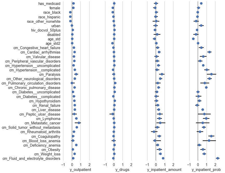
Here is a pictorial representation of the above two tables. The dots show the estimates and the horizontal line segments show the confidence intervals. This time, I haven't antilogged the coefficients, so the scale is visually symmetric for increases and decreases. (Antilogging numbers that range from -∞ to +∞ compresses the whole (-∞, 0) range to (0, 1) and further expands anything in (0, ∞).) And I excluded cm_Coagulopathy_hemophilia because it's so big it would require expanding the x-axis a lot just to accommodate it. Clearly, as in the tables, I'd need to clean up all the labels for publication.
Squared error
(display-pred-cv pred-cv-orx-rmse)
| I | DV | IVs | twin | RMSE |
|---|---|---|---|---|
| 0 | y_outpatient | trivial | single | 29,107 |
| 1 | y_outpatient | trivial | twin | 29,111 |
| 2 | y_outpatient | demog | single | 29,103 |
| 3 | y_outpatient | demog | twin | 29,111 |
| 4 | y_outpatient | demog+cm | single | 28,193 |
| 5 | y_outpatient | demog+cm | twin | 28,265 |
| 6 | y_drugs | trivial | single | 22,569 |
| 7 | y_drugs | trivial | twin | 22,533 |
| 8 | y_drugs | demog | single | 22,567 |
| 9 | y_drugs | demog | twin | 22,531 |
| 10 | y_drugs | demog+cm | single | 22,559 |
| 11 | y_drugs | demog+cm | twin | 22,526 |
Here I use lasso-regularized linear regression, and a multiplicative bias correction factor that I choose with another linear regression model in place of a smearing estimate or the normal bias correction factor or the like.
Here's what you'd get with OLS, without the lasso:
| I | DV | IVs | twin | RMSE |
|---|---|---|---|---|
| 0 | y_outpatient | trivial | single | 29,107 |
| 1 | y_outpatient | trivial | twin | 29,111 |
| 2 | y_outpatient | demog | single | 29,088 |
| 3 | y_outpatient | demog | twin | 29,104 |
| 4 | y_outpatient | demog+cm | single | 30,169 |
| 5 | y_outpatient | demog+cm | twin | 30,244 |
| 6 | y_drugs | trivial | single | 22,569 |
| 7 | y_drugs | trivial | twin | 22,533 |
| 8 | y_drugs | demog | single | 22,458 |
| 9 | y_drugs | demog | twin | 22,393 |
| 10 | y_drugs | demog+cm | single | 22,377 |
| 11 | y_drugs | demog+cm | twin | 22,381 |
Association of individual cost types
Here we have two tables of regression, one for each beneficiary status. Outpatient costs, inpatient costs (only among subjects with nonzero inpatient costs), drug costs, and subtotals (the sum of outpatient, inpatient, and drug costs) are fit with quantile regression: the central tendency is the median, the base error is the mean absolute deviation from the median (MAD) and the model error is the mean absolute error (MAE). The probability of nonzero inpatient costs is fit with logistic regression: the central tendency is the mean, the base error is the variance, and the model error is the mean squared error (i.e., the Brier score, which is a proper scoring rule; Brier, 1950; Bröcker, 2009).
For the quantile-regression models, the DVs are untransformed, so each coefficient can be interpreted directly as a linear increase of the conditional median, in dollars.
A few subjects were missing on the urban-rural variable. They were simply dropped.
Among Medicare beneficiaries, we only include subjects with Part D coverage for the full year.
Each row below "Intercept" shows the coefficient for the given variable. age_std is age standardized to have SD 1/2 (per Gelman, 2008), and age_std2 is its square, standardized again.
(display-assoc "mcare_only")
| I | subtotal | outpatient | inpatient_isnonzero | inpatient_nonzero | drugs |
|---|---|---|---|---|---|
| (n) | 1,551 | 1,551 | 1,551 | 183 | 1,551 |
| (central tendency) | 34,016 | 3,808 | 0.12 | 15,203 | 27,093 |
| (base error) | 18,482 | 6,324 | 0.10 | 18,425 | 11,932 |
| (model error) | 16,203 | 5,389 | 0.06 | 14,869 | 11,281 |
| Intercept | 19,166 | 894 | −3.62 | 22,879 | 23,241 |
| female | 50 | 348 | 1.18 | 115 | −4,339 |
| age_std | 1,991 | 336 | −0.46 | −373 | −851 |
| age_std2 | −2,031 | 213 | −0.44 | 2,509 | −4,673 |
| race_black | −5,277 | −968 | −0.33 | −3,376 | −4,969 |
| race_hispanic | −3,487 | −453 | −0.04 | 2,385 | −4,198 |
| race_other_nonwhite | −2,003 | −371 | −0.59 | −2,548 | −608 |
| urban | 4,608 | 1,110 | 0.18 | −15,012 | 1,729 |
| hiv_docvol_50plus | 2,246 | 173 | 0.02 | −2,427 | 2,556 |
| disabled | 5,719 | 352 | −0.28 | 4,695 | 937 |
| cm_Congestive_heart_failure | 3,176 | 857 | −0.21 | 4,331 | −539 |
| cm_Cardiac_arrhythmias | 7,122 | 2,890 | 1.47 | 6,490 | 1,553 |
| cm_Valvular_disease | 12,428 | 2,043 | 0.03 | 7,577 | 5,468 |
| cm_Peripheral_vascular_disorders | 1,664 | 1,431 | 0.19 | 10,999 | 247 |
| cm_Hypertension__uncomplicated | 2,092 | 521 | 0.78 | 975 | 1,159 |
| cm_Hypertension__complicated | 1,725 | 1,308 | 0.94 | −3,613 | −1,078 |
| cm_Paralysis | 33,092 | 5,713 | 3.11 | 4,841 | 1,152 |
| cm_Other_neurological_disorders | 5,711 | 2,401 | 1.14 | 2,748 | 1,810 |
| cm_Pulmonary_circulation_disorders | 18,202 | 5,635 | 2.57 | −894 | 3,046 |
| cm_Chronic_pulmonary_disease | 5,519 | 1,567 | 0.45 | 10,382 | 1,836 |
| cm_Diabetes__uncomplicated | 3,488 | 490 | 0.30 | −413 | 3,930 |
| cm_Diabetes__complicated | 8,099 | 2,404 | −1.35 | −496 | −266 |
| cm_Hypothyroidism | 8,869 | 2,156 | 1.05 | 443 | 2,125 |
| cm_Renal_failure | 3,892 | 1,719 | 0.32 | 2,724 | 244 |
| cm_Liver_disease | 2,575 | 1,649 | 0.36 | −2,368 | −284 |
| cm_Peptic_ulcer_disease | 2,511 | 0 | −12.88 | 0 | 2,871 |
| cm_Lymphoma | 12,123 | 6,075 | 0.45 | 23,220 | −4,035 |
| cm_Metastatic_cancer | 24,862 | 10,077 | 0.61 | 0 | −21 |
| cm_Solid_tumor_without_metastasis | 4,271 | 3,615 | 0.72 | 5,131 | 308 |
| cm_Rheumatoid_arthritis | 7,853 | 4,074 | 0.93 | −1,214 | 641 |
| cm_Coagulopathy | 7,510 | 2,391 | 1.98 | 8,816 | 1,029 |
| cm_Coagulopathy_hemophilia | 58,655 | 97,335 | 0.40 | 15,886 | 7,497 |
| cm_Blood_loss_anemia | 13,421 | 3,237 | 1.19 | 14,520 | 4,753 |
| cm_Deficiency_anemia | 3,748 | 736 | −0.23 | 29,003 | −379 |
| cm_Obesity | 7 | 1,089 | −0.16 | 23,943 | −5,062 |
| cm_Weight_loss | 9,330 | 1,762 | 0.90 | −384 | 3,017 |
| cm_Fluid_and_electrolyte_disorders | 13,241 | 3,773 | 3.02 | 1,062 | −2,818 |
(display-bnc "mcare_only")
| n_comorbs | subjects | median_subtotal |
|---|---|---|
| 0 | 536 | 27,777 |
| 1 | 461 | 33,427 |
| 2 | 252 | 37,191 |
| 3 | 138 | 37,552 |
| 4 | 52 | 42,583 |
| 5 | 43 | 49,880 |
| 6 | 28 | 74,897 |
| 7 | 21 | 67,386 |
| ≥ 8 | 20 | 112,836 |
(display-assoc "dual")
| I | subtotal | outpatient | inpatient_isnonzero | inpatient_nonzero | drugs |
|---|---|---|---|---|---|
| (n) | 6,137 | 6,137 | 6,137 | 1,242 | 6,137 |
| (central tendency) | 35,630 | 4,674 | 0.20 | 18,692 | 27,347 |
| (base error) | 25,091 | 7,444 | 0.16 | 29,595 | 13,295 |
| (model error) | 20,224 | 5,901 | 0.10 | 25,463 | 12,920 |
| Intercept | 26,602 | 2,447 | −2.95 | 4,919 | 23,926 |
| female | −1,234 | 970 | 0.12 | −763 | −2,407 |
| age_std | −1,060 | −91 | −0.47 | −3,166 | 538 |
| age_std2 | −4,113 | −63 | 0.17 | 12 | −2,803 |
| race_black | −3,072 | −404 | 0.04 | −877 | −3,308 |
| race_hispanic | −1,153 | −459 | −0.04 | 1,078 | −1,055 |
| race_other_nonwhite | 354 | −96 | 0.01 | −315 | 670 |
| urban | 2,962 | −292 | 0.10 | 3,097 | 1,116 |
| hiv_docvol_50plus | 211 | 174 | −0.13 | 10 | 1,294 |
| disabled | −971 | 224 | −0.00 | −1,842 | 810 |
| cm_Congestive_heart_failure | 11,874 | 3,107 | 0.39 | 4,336 | −1,170 |
| cm_Cardiac_arrhythmias | 10,714 | 3,127 | 1.14 | 6,130 | 195 |
| cm_Valvular_disease | 15,066 | 5,068 | 0.65 | 14,762 | 406 |
| cm_Peripheral_vascular_disorders | 11,217 | 3,283 | 0.14 | 8,595 | 2,559 |
| cm_Hypertension__uncomplicated | 2,944 | 878 | 0.70 | 2,925 | 1,202 |
| cm_Hypertension__complicated | 14,482 | 5,381 | 0.97 | 3,746 | −163 |
| cm_Paralysis | 21,317 | 5,188 | 1.06 | 6,961 | 2,361 |
| cm_Other_neurological_disorders | 16,184 | 3,367 | 1.51 | 8,319 | 1,875 |
| cm_Pulmonary_circulation_disorders | 18,709 | 3,687 | −0.00 | 10,189 | 5,691 |
| cm_Chronic_pulmonary_disease | 7,827 | 2,356 | 1.14 | 2,334 | 1,800 |
| cm_Diabetes__uncomplicated | 2,705 | 435 | 0.14 | −1,572 | 2,745 |
| cm_Diabetes__complicated | 8,199 | 2,768 | 0.16 | 4,942 | 479 |
| cm_Hypothyroidism | 4,939 | 1,488 | 0.28 | −3,439 | 3,123 |
| cm_Renal_failure | 6,878 | 1,849 | −0.12 | 4,742 | 1,254 |
| cm_Liver_disease | 5,160 | 1,785 | 0.62 | 3,092 | 1,041 |
| cm_Peptic_ulcer_disease | 19,533 | 5,758 | 1.13 | 54,846 | −3,050 |
| cm_Lymphoma | 9,799 | 2,303 | 0.88 | 3,007 | −1,233 |
| cm_Metastatic_cancer | 30,821 | 14,990 | 1.41 | 2,750 | 1,361 |
| cm_Solid_tumor_without_metastasis | 9,499 | 4,782 | 0.57 | 5,440 | 1,195 |
| cm_Rheumatoid_arthritis | 3,466 | 1,216 | −0.15 | −221 | 1,750 |
| cm_Coagulopathy | 20,571 | 2,699 | 1.35 | 13,974 | −2,334 |
| cm_Coagulopathy_hemophilia | 170,713 | 79,780 | −0.23 | 16,538 | 12,508 |
| cm_Blood_loss_anemia | 8,795 | 4,863 | 1.26 | 12,058 | −1,788 |
| cm_Deficiency_anemia | 11,435 | 4,041 | 0.07 | 4,719 | 2,502 |
| cm_Obesity | 3,297 | 156 | 0.78 | 4,450 | 434 |
| cm_Weight_loss | 17,755 | 2,807 | 0.76 | 12,035 | 3,392 |
| cm_Fluid_and_electrolyte_disorders | 18,912 | 3,560 | 2.39 | 4,532 | −1,214 |
(display-bnc "dual")
| n_comorbs | subjects | median_subtotal |
|---|---|---|
| 0 | 2,208 | 28,840 |
| 1 | 1,539 | 34,133 |
| 2 | 950 | 39,367 |
| 3 | 531 | 47,967 |
| 4 | 305 | 56,389 |
| 5 | 205 | 62,527 |
| 6 | 131 | 88,344 |
| 7 | 93 | 100,588 |
| 8 | 58 | 116,936 |
| 9 | 35 | 115,445 |
| 10 | 29 | 164,307 |
| 11 | 17 | 223,938 |
| 12 | 19 | 190,814 |
| ≥ 13 | 17 | 274,452 |
Methods paper
If we chose models on the basis of fit rather than predictive accuracy, then we know a priori that the most complex models would win. This means that for outpatient and drug costs, twin models with all IVs would win (which is similar to the real winning models, non-twin with all IVs), whereas for inpatient costs, all IVs would win (which is the same result we got with predictive accuracy).
We might also compare model selection based on predictive accuracy to model selection based on p-values. In particular, we can use the simple-minded method of trying all the predictors and keeping the significant ones. But how shall I test the significance of the coefficients? quantreg doesn't supply significance tests for models fit with a lasso penalty. Let's use the method of Redden, Fernández, and Allison (2004).
Scott: "Thinking of discussion points: Predictive analytics have not been big in HIV research in part because of smaller data sets we typically collect. However, large data sets, such as Medicaid / Medicare data, are becoming more of the norm than the exception in HIV research. Think of ATN and other large scale studies. NIH push to make data sets publicly available. Virtual cohorts with medical chart data. Basically, predictive analytic tools are needed."
Rob suggested trying a Box-Cox, but this would probably be a hassle to use with quantile regression or lasso linear regression, because it means there's another kind of parameter to fit. Besides, Box-Cox sort of ruins the interpretability of the coefficients, so it's not a good choice when coefficient interpretation is a goal.
I found that I wasn't able to get the sort of improvements on square error that I was able to get on absolute error. My impression is that this is basically a consequence of the high skew of the DVs: a few high values affect square error more than absolute error, so models that optimize mean square error will make a stupider sort of compromise than models that optimize absolute error. This could be discussed in the method paper with a simple, mathematically clean example, and with the RMSEs for outpatient costs.
Outline
- Describe prediction and contrast it with association (as in Arfer & Luhmann, 2017)
- Describe the method I used in the first paper on Comorbid
- Contrast the models thus selected with those that would be selected if we just fit models with all the IVs and then dropped IVs with non-significant coefficients
- We can contrast the models in terms of predictive accuracy as well as just the coefficients
- Contrast the fits of the models with their predictive accuracies
- Discussion: predictive methods are more useful these days now that large datasets are more widely available (e.g., the ATN, virtual cohorts with medical charts, increasing interest in making datasets publicly accessible)
References
Arfer, K. B., & Luhmann, C. C. (2017). Time-preference tests fail to predict behavior related to self-control. Frontiers in Psychology, 8(150). doi:10.3389/fpsyg.2017.00150
Brier, G. W. (1950). Verification of forecasts expressed in terms of probability. Monthly Weather Review, 78(1), 1–3. doi:10.1175/1520-0493(1950)078<0001:VOFEIT>2.0.CO;2
Bröcker, J. (2009). Reliability, sufficiency, and the decomposition of proper scores. Quarterly Journal of the Royal Meteorological Society, 135(643), 1512–1519. doi:10.1002/qj.456
Buntin, M. B., & Zaslavsky, A. M. (2004). Too much ado about two-part models and transformation? Journal of Health Economics, 23(3), 525–542. doi:10.1016/j.jhealeco.2003.10.005
Gelman, A. (2008). Scaling regression inputs by dividing by two standard deviations. Statistics in Medicine, 27(15), 2865–2873. doi:10.1002/sim.3107
Newman, M. C. (1993). Regression analysis of log-transformed data: Statistical bias and its correction. Environmental Toxicology and Chemistry, 12(6), 1129–1133. doi:10.1002/etc.5620120618
Redden, D. T., Fernández, J. R., & Allison, D. B. (2004). A simple significance test for quantile regression. Statistics in Medicine, 23(16), 2587–2597. doi:10.1002/sim.1839