mSTUDY notebook
Created 24 Sep 2016 • Last modified 31 Jan 2019
General information
Go to Amy Ragsdale for questions about the data.
None of the subjects use injection drugs.
Viral load level
From: Brendan Quinn
Date: 14 September 2016
To: Jesse L. ClarkI'm working on a HIV paper with Steve Shoptaw and he asked me to get in touch with you to ask what level you would use for undetectable viral load?
From: Jesse L. Clark
Date: 14 September 2016
To: Brendan QuinnIt depends on the machine used for testing. The standard we use at ucla has a lower limit of detection of 20 copies per mL. The machines commonly used in South America have a limit of 50 copies. In the past (about 10 or 15 years ago) the standard lower limit was 400 copies. If you are using recent data from a developed country setting you should be safe assuming the upper limit of detection is 20 copies per mL.
Thinking
The first kind of DV to consider is HIV transmission risk.
- In HIV-positive subjects, this is viral load (dichotomized as detectable or undetectable)
- In HIV-negative subjects, this is receptive anal sex with an HIV-positive or HIV-unknown partner (ideally, we would focus on unprotected such sex, but that wasn't measured)
Possible framings of the problem:
- Use only the DVs in the last timepoint available for each subject as the DV to be predicted. (So the DVs at previous timepoints are essentially IVs, from the perspective of the predictive procedure.)
- Treat every timepoint as a potential case to be predicted, but allow the model to see all past timepoints. This rules out conventional k-fold cross-validation (if in one fold you have timepoint 1 in training and timepoint 2 in testing, you'll have it the other way around in another fold). I guess the simplest way to do this is a variation on leave-one-out where we consider one observation at a time and allow everything as training data except that observation and future observations for the same subject.
Model extensions to consider:
- Age and race
Simple analyses
Race
(setv d (.append
  (.mean
    (getl obs1 : (filt (.startswith it "race_") obs1.columns)))
  (pd.Series :index ["race_hispanic"] (.mean
    (= (ss ($ obs1 race_hispanic) (pd.notnull $)) "Yes")))))
(rd 2 (.sort-values d :ascending F))
| I | value |
|---|---|
| race_hispanic | 0.49 |
| race_black | 0.45 |
| race_white | 0.31 |
| race_nat_am | 0.07 |
| race_asian | 0.02 |
| race_pacific | 0.02 |
| race_indian | 0.01 |
Only black, Hispanic, and white have sufficiently high prevalences for them to have much predictive value.
Age
(setv v (valcounts (.astype (ss ($ obs1 age_at_baseline) (pd.notnull $)) int)))
(plt.bar (- v.index .5) v.values :width 1 :color "black" :edgecolor "none")
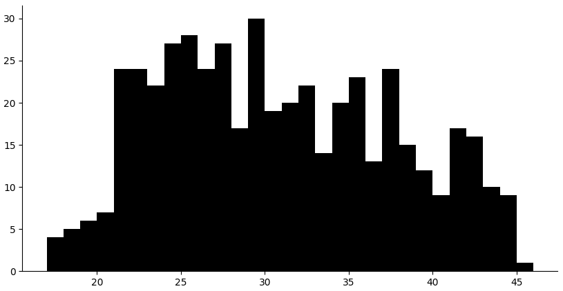
Looks okay.
Rates of self-reported drug usage
(setv d (. (.apply (.groupby obs "hiv_status") (λ
  (.mean (~ (.isin
    (getl it : (filt (.startswith it "drug_sr_") it.columns))
    (qw Never Once)))))) T))
(rd 2 (ordf d (.mean d 1)))
| I | HIV- | HIV+ |
|---|---|---|
| drug_sr_heroin | 0.04 | 0.01 |
| drug_sr_other | 0.05 | 0.02 |
| drug_sr_crack | 0.07 | 0.04 |
| drug_sr_mdma | 0.09 | 0.06 |
| drug_sr_party | 0.06 | 0.12 |
| drug_sr_rx | 0.13 | 0.06 |
| drug_sr_pde5_inhib | 0.10 | 0.10 |
| drug_sr_powder_cocaine | 0.15 | 0.08 |
| drug_sr_alkyl_nitrite | 0.22 | 0.25 |
| drug_sr_meth | 0.22 | 0.47 |
| drug_sr_cigarettes | 0.46 | 0.47 |
| drug_sr_cannabis | 0.51 | 0.44 |
| drug_sr_alcohol_heavy | 0.61 | 0.46 |
| drug_sr_alcohol | 0.81 | 0.72 |
Here's the proportion of observations at which a subject had used the drug in question more than once (or for the alcohol items, even once). Only a few (alkyl nitrite, meth, cigarettes, cannabis, and alcohol) have usage in more than a fifth of observations in either group. Another four drugs (PDE5 inhibitors, other party drugs, perscription drugs, and powder cocaine) have usage between 10% and 20% in at least one of the two groups. Two of these drugs (other party drugs and perscription drugs) are rather vague classes of drugs and hence seem unlikely to be useful for analysis. In summary, we should probably concern ourselves with alcohol, cannabis, cigarettes, meth, alklyl nitrite, powder cocaine, and PDE5 inhibitors.
(rd 2 (.apply (.groupby obs "hiv_status") (λ
  (.mean (.any (~ (.isin
    (getl it : (qw
      drug_sr_heroin drug_sr_other drug_sr_crack drug_sr_mdma drug_sr_party drug_sr_rx))
    (qw Never Once))) :axis 1)))))
| hiv_status | value |
|---|---|
| HIV- | 0.23 |
| HIV+ | 0.22 |
Here's the proportion of subjects who used at least one of these rarer drugs more than once.
Urine tests
(setv obs-good (ss obs (.isin $s s-good)))
(setv d (. (pd.concat :axis 1 (rmap [[sr urine] [
    ["drug_sr_meth" "drug_urine_meth"]
    ["drug_sr_mdma" "drug_urine_mdma"]
    ["drug_sr_cannabis" "drug_urine_cannabis"]
    [["drug_sr_powder_cocaine" "drug_sr_crack"] "drug_urine_cocaine"]
    ["drug_sr_heroin" "drug_urine_opiate"]
    ["drug_sr_alkyl_nitrite" "drug_urine_nitrite"]]]
  (setv deny (if (coll? sr)
    (.all (= (getl obs-good : sr) "Never") :axis 1)
    (= (getl obs-good : sr) "Never")))
  (valcounts (getl (get obs-good deny) : urine)))) T))
(setv ($ d prop) (rd 2 (wc d (/ $Positive (+ $Positive $Negative)))))
(getl (.rename d :index (λ (cut it (len "drug_urine_")))) :
  (qw N/A Positive Negative prop))
| I | N/A | Positive | Negative | prop |
|---|---|---|---|---|
| meth | 2 | 23 | 801 | 0.03 |
| mdma | 5 | 36 | 1116 | 0.03 |
| cannabis | 4 | 71 | 569 | 0.11 |
| cocaine | 4 | 8 | 1046 | 0.01 |
| opiate | 5 | 14 | 1275 | 0.01 |
| nitrite | 4 | 13 | 898 | 0.01 |
This shows the urine tests results among observations for which the subject denied using each drug. These dishonesty rates are pretty low. The one for cannabis is probably higher because physiological tests for cannabis have much longer temporal ranges than those for other drugs.
There's some slippage for heroin because heroin isn't actually an opiate, just an opioid, so I don't know if the opiate urine test could in fact detect it.
(setv d (pd.DataFrame :columns (qw drug n prop) (rmap [[sr urine] [
    ["drug_sr_meth" "drug_urine_meth"]
    ["drug_sr_mdma" "drug_urine_mdma"]
    ["drug_sr_cannabis" "drug_urine_cannabis"]
    [["drug_sr_powder_cocaine" "drug_sr_crack"] "drug_urine_cocaine"]
    ["drug_sr_heroin" "drug_urine_opiate"]
    ["drug_sr_alkyl_nitrite" "drug_urine_nitrite"]]]
  (setv o (.dropna (getl obs : (+
    (if (coll? sr) sr [sr]) [urine]))))
  (setv admit (~ (if (coll? sr)
    (.all (= (getl o : sr) "Never") :axis 1)
    (= (getl o : sr) "Never"))))
  [urine (len o) (.mean (= admit (= (getl o : urine) "Positive")))])))
(rd 2 (.rename (.set-index d "drug")
  :index (λ (cut it (len "drug_urine_")))))
| drug | n | prop |
|---|---|---|
| meth | 1350 | 0.76 |
| mdma | 1350 | 0.84 |
| cannabis | 1350 | 0.72 |
| cocaine | 1350 | 0.82 |
| opiate | 1350 | 0.96 |
| nitrite | 1350 | 0.68 |
This table shows the proportion of observations for which self-report agreed with urine tests (among observations for which neither is missing).
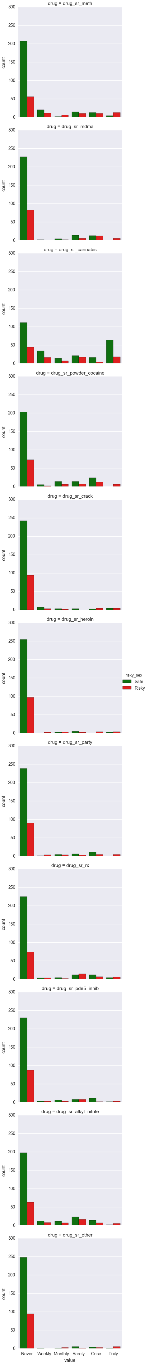
Cross-tabulation of self-reported drug usage and the DV
HIV-negative
(setv d (pd.melt :id_vars ["risky_sex"] :var_name "drug"
  (getl obs-hiv- : (+ ["risky_sex"] (filt
    (and (.startswith it "drug_sr_") (not-in "alcohol" it) (not-in "cigarettes" it))
    obs.columns)))))

(sns.factorplot :data d :kind "count"
  :row "drug" :x "value" :hue "risky_sex"
  :hue_order (qw Safe Risky)
  :palette {"Risky" "red" "Safe" "green"})
(setv l (rmap [dc (filt
    (and (.startswith it "drug_sr_") (not-in "alcohol" it) (not-in "cigarettes" it)) obs.columns)]
  (setv x (.apply (.groupby obs-hiv- dc) (λ
    (.mean (= ($ it risky_sex) "Risky")))))
  (setv x.name (cut x.index.name (len "drug_sr_")))
  x))
(rd 2 (pd.DataFrame l))
| I | Never | Once | Rarely | Monthly | Weekly | Daily |
|---|---|---|---|---|---|---|
| meth | 0.20 | 0.43 | 0.37 | 0.60 | 0.35 | 0.72 |
| mdma | 0.25 | 0.48 | 0.25 | 0.25 | 0.00 | 0.83 |
| cannabis | 0.26 | 0.18 | 0.45 | 0.33 | 0.30 | 0.21 |
| powder_cocaine | 0.25 | 0.33 | 0.30 | 0.29 | 0.20 | 1.00 |
| crack | 0.26 | 0.67 | 0.00 | 0.25 | 0.27 | 0.50 |
| heroin | 0.26 | 0.60 | 0.20 | 0.67 | 1.00 | 0.60 |
| party | 0.26 | 0.25 | 0.25 | 0.43 | 0.75 | 0.80 |
| rx | 0.23 | 0.37 | 0.52 | 0.33 | 0.50 | 0.50 |
| pde5_inhib | 0.26 | 0.15 | 0.50 | 0.27 | 0.50 | 0.50 |
| alkyl_nitrite | 0.22 | 0.32 | 0.40 | 0.39 | 0.40 | 0.62 |
| other | 0.26 | 0.38 | 0.14 | 0.75 | 0.00 | 0.71 |
(rd 2 (.apply (.groupby obs-hiv- "drug_sr_alcohol") (λ
  (.mean (= ($ it risky_sex) "Risky")))))
| drug_sr_alcohol | value |
|---|---|
| Never | 0.29 |
| Monthly or less | 0.24 |
| 2 to 4 times a month | 0.27 |
| 2 to 3 times a week | 0.29 |
| 4 or more times a week | 0.30 |
(rd 2 (.apply (.groupby obs-hiv- "drug_sr_alcohol_heavy") (λ
  (.mean (= ($ it risky_sex) "Risky")))))
| drug_sr_alcohol_heavy | value |
|---|---|
| Never | 0.26 |
| Less than monthly | 0.23 |
| Monthly | 0.37 |
| Weekly | 0.27 |
| Daily or almost daily | 0.32 |
(rd 2 (.apply (.groupby obs-hiv- "drug_sr_cigarettes") (λ
  (.mean (= ($ it risky_sex) "Risky")))))
| drug_sr_cigarettes | value |
|---|---|
| Never | 0.25 |
| Occasionally(<1 cigarette/day) | 0.30 |
| Less than half pack/day | 0.35 |
| At least half pack, but less than 1 pack/day | 0.14 |
| 1 pack/day or more, but less than 2 packs/day | 0.39 |
| 2+ packs/day | 0.50 |
Daily usage of any drug (other than cannabis or alcohol), although uncommon, seems particularly associated with risky sex.
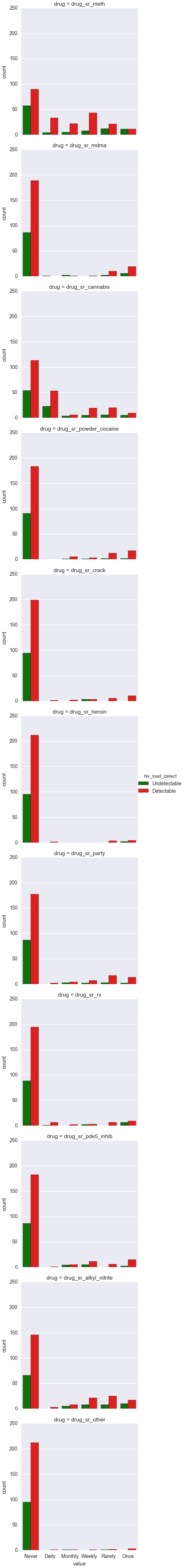
HIV-positive
(setv d (pd.melt :id_vars ["hiv_load_detect"] :var_name "drug"
  (getl obs-hiv+ : (+ ["hiv_load_detect"] (filt
    (and (.startswith it "drug_sr_") (not-in "alcohol" it) (not-in "cigarettes" it))
    obs.columns)))))

(sns.factorplot :data d :kind "count"
  :row "drug" :x "value" :hue "hiv_load_detect"
  :hue_order (qw Undetectable Detectable)
  :palette {"Detectable" "red" "Undetectable" "green"})
(setv l (rmap [dc (filt
    (and (.startswith it "drug_sr_") (not-in "alcohol" it) (not-in "cigarettes" it)) obs.columns)]
  (setv x (.apply (.groupby obs-hiv+ dc) (λ
    (.mean (= ($ it hiv_load_detect) "Detectable")))))
  (setv x.name (cut x.index.name (len "drug_sr_")))
  x))
(rd 2 (pd.DataFrame l))
| I | Never | Once | Rarely | Monthly | Weekly | Daily |
|---|---|---|---|---|---|---|
| meth | 0.61 | 0.50 | 0.64 | 0.79 | 0.80 | 0.89 |
| mdma | 0.68 | 0.76 | 0.83 | 0.33 | 1.00 | 0.00 |
| cannabis | 0.68 | 0.64 | 0.77 | 0.55 | 0.79 | 0.67 |
| powder_cocaine | 0.66 | 0.85 | 0.86 | 0.83 | 0.75 | |
| crack | 0.67 | 0.91 | 1.00 | 1.00 | 0.50 | 1.00 |
| heroin | 0.68 | 0.67 | 1.00 | 1.00 | ||
| party | 0.67 | 0.87 | 0.81 | 0.50 | 0.78 | 1.00 |
| rx | 0.68 | 0.60 | 1.00 | 1.00 | 0.50 | 0.86 |
| pde5_inhib | 0.67 | 0.83 | 1.00 | 0.56 | 0.69 | 1.00 |
| alkyl_nitrite | 0.69 | 0.61 | 0.74 | 0.62 | 0.70 | 1.00 |
| other | 0.68 | 1.00 | 0.67 | 0.50 | 1.00 | 1.00 |
(rd 2 (.apply (.groupby obs-hiv+ "drug_sr_alcohol") (λ
  (.mean (= ($ it hiv_load_detect) "Detectable")))))
| drug_sr_alcohol | value |
|---|---|
| Never | 0.58 |
| Monthly or less | 0.66 |
| 2 to 4 times a month | 0.79 |
| 2 to 3 times a week | 0.76 |
| 4 or more times a week | 0.71 |
(rd 2 (.apply (.groupby obs-hiv+ "drug_sr_alcohol_heavy") (λ
  (.mean (= ($ it hiv_load_detect) "Detectable")))))
| drug_sr_alcohol_heavy | value |
|---|---|
| Never | 0.64 |
| Less than monthly | 0.78 |
| Monthly | 0.77 |
| Weekly | 0.70 |
| Daily or almost daily | 0.55 |
(rd 2 (.apply (.groupby obs-hiv+ "drug_sr_cigarettes") (λ
  (.mean (= ($ it hiv_load_detect) "Detectable")))))
| drug_sr_cigarettes | value |
|---|---|
| Never | 0.63 |
| Occasionally(<1 cigarette/day) | 0.68 |
| Less than half pack/day | 0.79 |
| At least half pack, but less than 1 pack/day | 0.78 |
| 1 pack/day or more, but less than 2 packs/day | 0.54 |
| 2+ packs/day |
(Blank cells in the tables mean there were no HIV+ subjects with that level of drug use.)
These results overall look similar to the one for HIV- subjects and risky sex. Most drugs, the chief exceptions being alcohol and cigarettes, are associated with higher viral load at higher doses.
Prediction
HIV-negative
(setv results-freq (pred "risky_sex_receive" "Risky" "freq" obs-hiv-))
(show-pred-table results-freq)
| I | MSE | p when y=0 | p when y=1 |
|---|---|---|---|
| trivial-between | 0.20674 | 0.290 | 0.287 |
| trivial-within | 0.20762 | 0.276 | 0.328 |
| logistic | 0.20325 | 0.275 | 0.327 |
| logistic-ridge | 0.19846 | 0.279 | 0.315 |
| logistic-lasso | 0.19629 | 0.283 | 0.333 |
| I | MSE | p when y=0 | p when y=1 |
|---|---|---|---|
| trivial-between | 0.20674 | 0.290 | 0.287 |
| trivial-within | 0.20762 | 0.276 | 0.328 |
| logistic | 0.20165 | 0.273 | 0.331 |
| logistic-ridge | 0.19860 | 0.279 | 0.317 |
| logistic-lasso | 0.19634 | 0.283 | 0.332 |
| logistic-random | 0.20065 | 0.244 | 0.318 |
This table uses dose-response models. The mean squared error (MSE) is from a variation on leave-one-out cross-validation. The drugs items are coded as monthly frequencies.
All the regression models do better than the trivial models (with don't use any of the predictors, except for subject for trivial-within). The best performer is logistic-lasso, which is logistic regression with a lasso (L1) penalty.
(setv results-binary (pred "risky_sex_receive" "Risky" "any_or_none" obs-hiv-))
(show-pred-table results-binary)
| I | MSE | p when y=0 | p when y=1 |
|---|---|---|---|
| trivial-between | 0.20674 | 0.290 | 0.287 |
| trivial-within | 0.20762 | 0.276 | 0.328 |
| logistic | 0.19973 | 0.266 | 0.341 |
| logistic-ridge | 0.20916 | 0.292 | 0.300 |
| logistic-lasso | 0.25219 | 0.421 | 0.381 |
| logistic-random | 0.19987 | 0.247 | 0.330 |
This table is similar but uses dichotomous models, where each drug was dichotomized as any use vs. no use.
Here, curiously, the penalized regression models underperform the trivial models. The best is logistic.
So the best-performing dose-response model (logistic-lasso, MSE .196) does slightly better than the best-performing binary model (logistic, MSE .200).
(plt.xlim [0 1])
(sns.kdeplot (get results-freq "ypp" "logistic-lasso") :bw .1
  :label "freq")
(sns.kdeplot (get results-binary "ypp" "logistic") :bw .1
  :label "binary")
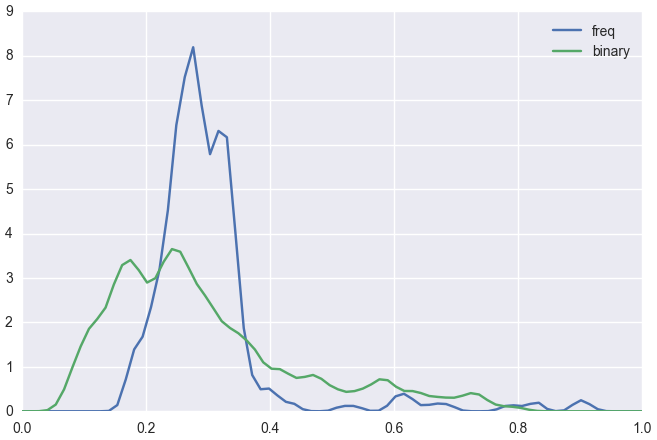
Here is a density plot of the predicted probabilities across all observations, comparing the best-performing dose-response model to the best-performing binary model. The dose-response model is simpler in the sense that it outputs a smaller range of probabilities. This may be due to the effect of the lasso.
(.map
  (pd.Series
    (get results-freq "coefs_all_obs" "logistic-lasso")
    :index (+ ["Intercept"]
      (filt (!= it "s") (get results-freq "x_vars"))))
  (λ (if (= it 0) "" (format it ".3f"))))
| I | value |
|---|---|
| Intercept | -0.687 |
| t | |
| race_white | |
| race_black | -0.283 |
| race_other | -0.048 |
| age_at_baseline | -0.216 |
| drug_sr_alcohol | |
| drug_sr_alcohol_heavy | |
| drug_sr_cigarettes | |
| drug_sr_cannabis | -0.310 |
| drug_sr_meth | 0.675 |
| drug_sr_alkyl_nitrite | |
| drug_sr_powder_cocaine | 0.461 |
| drug_sr_pde5_inhib |
Here are the coefficients of the dose-response model. Several coefficients are 0 (shown as blank) because of the lasso penalty. t is the effect of time. Drug frequencies and age were standardized to have SD 1/2. Since this is a logistic-regression model, the coefficients are on the scale of log odds ratios.
We see that both powder cocaine and methamphetamine are associated with a higher probability of risky sex the more they are used. For cannabis, there's a negative effect.
HIV-positive: risky sex
(setv results-freq (pred "risky_sex_transmit_d" "Risky" "freq" obs-hiv+))
(show-pred-table results-freq)
| I | MSE | p when y=0 | p when y=1 |
|---|---|---|---|
| trivial-between | 0.20248 | 0.280 | 0.276 |
| trivial-within | 0.20837 | 0.279 | 0.313 |
| logistic | 0.20799 | 0.275 | 0.292 |
| logistic-ridge | 0.20440 | 0.282 | 0.275 |
| logistic-lasso | 0.25052 | 0.500 | 0.498 |
| logistic-random | 0.20828 | 0.246 | 0.270 |
(setv results-binary (pred "risky_sex_transmit_d" "Risky" "any_or_none" obs-hiv+))
(show-pred-table results-binary)
| I | MSE | p when y=0 | p when y=1 |
|---|---|---|---|
| trivial-between | 0.20248 | 0.280 | 0.276 |
| trivial-within | 0.20837 | 0.279 | 0.313 |
| logistic | 0.20369 | 0.268 | 0.308 |
| logistic-ridge | 0.20322 | 0.281 | 0.276 |
| logistic-lasso | 0.25000 | 0.500 | 0.500 |
| logistic-random | 0.20461 | 0.250 | 0.292 |
trivial-between is the winner among both the dose-response and binary models.
HIV-positive: viral load detectability
(setv results-freq (pred "hiv_load_detect" "Detectable" "freq" obs-hiv+))
(show-pred-table results-freq)
| I | MSE | p when y=0 | p when y=1 |
|---|---|---|---|
| trivial-between | 0.21398 | 0.697 | 0.693 |
| trivial-within | 0.20034 | 0.668 | 0.739 |
| logistic | 0.21984 | 0.678 | 0.697 |
| logistic-ridge | 0.21913 | 0.700 | 0.691 |
| logistic-lasso | 0.21842 | 0.629 | 0.625 |
| logistic-random | 0.20929 | 0.684 | 0.770 |
Here the winner is a trivial model, trivial-within.
(setv results-binary (pred "hiv_load_detect" "Detectable" "any_or_none" obs-hiv+))
(show-pred-table results-binary)
| I | MSE | p when y=0 | p when y=1 |
|---|---|---|---|
| trivial-between | 0.21398 | 0.697 | 0.693 |
| trivial-within | 0.20034 | 0.668 | 0.739 |
| logistic | 0.21466 | 0.667 | 0.705 |
| logistic-ridge | 0.21096 | 0.671 | 0.704 |
| logistic-lasso | 0.20972 | 0.662 | 0.703 |
| logistic-random | 0.20561 | 0.669 | 0.777 |
trivial-within is again the best performer.
Indicator models
Here I take the approach suggested by Ron Brookmeyer of using dummy variables for the various possible responses to the drug-use questions, and looking at the coefficients to decide whether there's a dose-response effect.
Data setup
First we should check which response choices are rare enough that they should be collapsed with others. We're restricting our attention to binge drinking (not any drinking), methamphetamine, cannabis, and alkyl nitrites (per Steve).
(setv d (ss obs (.isin $s s-good)))
(setv d (pd.concat :axis 1 (rmap [drug (qw meth cannabis alkyl_nitrite)]
  (valcounts
    (getl d : (+ "drug_sr_" drug))
    (+ drug " " (.astype ($ d hiv_status) str))))))
(setv d.index.name "I")
(setv d.columns (amap
  (-> it
    (.replace "cannabis" "weed")
    (.replace "alkyl_nitrite" "pop")
    (.replace "HIV" "H"))
  d.columns))
d
| I | meth H+ | meth H- | weed H+ | weed H- | pop H+ | pop H- |
|---|---|---|---|---|---|---|
| Never | 325 | 483 | 357 | 276 | 430 | 468 |
| Once | 50 | 36 | 28 | 44 | 48 | 38 |
| Less than monthly | 69 | 39 | 49 | 66 | 72 | 64 |
| Monthly | 55 | 14 | 28 | 34 | 40 | 27 |
| Weekly | 97 | 45 | 47 | 87 | 66 | 36 |
| Daily | 73 | 33 | 160 | 143 | 13 | 17 |
For alkyl nitrites (poppers), Daily should probably be combined with Weekly. All the other categories seem reasonably sized except for Monthly for metamphetamine among HIV-negatives, but among HIV-positives this isn't the case, and it will probably be simpler to use the same coding for both HIV statuses.
(wc (ss obs (.isin $s s-good))
  (valcounts $drug_sr_alcohol_heavy $hiv_status))
| drug_sr_alcohol_heavy | HIV- | HIV+ |
|---|---|---|
| Never | 256 | 381 |
| Less than monthly | 184 | 147 |
| Monthly | 94 | 66 |
| Weekly | 84 | 54 |
| Daily or almost daily | 32 | 21 |
Looks okay.
(setv d-ind (.reset-index :drop T (ss obs (.isin $s s-good) (qw
  risky_sex_receive
  risky_sex_transmit_d
  hiv_load_detect
  s
  hiv_status
  interviewed
  race_hispanic
  race_black
  race_white
  age_at_baseline
  used_prep
  drug_sr_alcohol_heavy
  drug_sr_cannabis
  drug_sr_alkyl_nitrite
  drug_sr_meth))))

(setv baseline-interview
  (.apply (.groupby d-ind "s") (λ (.min ($ it interviewed)))))
(setv ($ d-ind years_since_baseline) (wc d-ind
  (/ (. (- $interviewed (.map $s baseline-interview)) dt days) 365.25)))
(setv d-ind (.drop d-ind :columns "interviewed"))
(setv ($ d-ind years2_since_baseline) (** ($ d-ind years_since_baseline) 2))

(setv (get d-ind.loc (, (= ($ d-ind drug_sr_alkyl_nitrite) "Daily") "drug_sr_alkyl_nitrite"))
  "Weekly")
(setv ($ d-ind drug_sr_alkyl_nitrite) (-> ($ d-ind drug_sr_alkyl_nitrite)
  (.cat.rename-categories {"Weekly" "Daily or weekly"})
  (.cat.remove-categories ["Daily"])))

(setv ($ d-ind race_hispanic) (= ($ d-ind race_hispanic) "Yes"))
(setv ($ d-ind used_prep) (= ($ d-ind used_prep) "YesPrEP"))

(setv d-ind-xvars (->> d-ind.columns (filt (not-in it [
  "hiv_status"
  "risky_sex_receive" "risky_sex_transmit_d" "hiv_load_detect"]))))

d-ind.shape
| 1338 | 16 |
Results
Here we have odds ratios and 95% confidence intervals thereof, as tables and plots. (The plots have logged x-axes.) I consider the question of whether each drug seems to have a dose-response effect.
(rd 2 (digest-indicator (go-indicator
  d "HIV-" "risky_sex_receive" "Risky")))
| I | point | lo | hi |
|---|---|---|---|
| (Intercept) | 0.17 | 0.04 | 0.92 |
| race_hispanic: TRUE | 1.56 | 0.74 | 3.37 |
| race_black: TRUE | 0.76 | 0.31 | 1.51 |
| race_white: TRUE | 1.05 | 0.51 | 2.00 |
| age_at_baseline | 0.99 | 0.95 | 1.03 |
| years_since_baseline | 1.00 | 0.41 | 2.51 |
| years2_since_baseline | 1.05 | 0.69 | 1.55 |
| drug_sr_alcohol_heavy: Less than monthly | 0.74 | 0.36 | 1.37 |
| drug_sr_alcohol_heavy: Monthly | 1.21 | 0.53 | 2.51 |
| drug_sr_alcohol_heavy: Weekly | 1.11 | 0.50 | 2.82 |
| drug_sr_alcohol_heavy: Daily or almost daily | 1.03 | 0.28 | 3.55 |
| drug_sr_cannabis: Once | 0.83 | 0.29 | 2.18 |
| drug_sr_cannabis: Less than monthly | 1.65 | 0.70 | 4.12 |
| drug_sr_cannabis: Monthly | 0.88 | 0.22 | 2.74 |
| drug_sr_cannabis: Weekly | 0.73 | 0.31 | 1.54 |
| drug_sr_cannabis: Daily | 0.83 | 0.40 | 1.63 |
| drug_sr_alkyl_nitrite: Once | 1.57 | 0.53 | 4.21 |
| drug_sr_alkyl_nitrite: Less than monthly | 2.39 | 1.05 | 5.50 |
| drug_sr_alkyl_nitrite: Monthly | 2.46 | 0.79 | 7.89 |
| drug_sr_alkyl_nitrite: Daily or weekly | 2.63 | 1.03 | 6.61 |
| drug_sr_meth: Once | 1.51 | 0.42 | 4.21 |
| drug_sr_meth: Less than monthly | 3.03 | 1.08 | 8.69 |
| drug_sr_meth: Monthly | 3.56 | 0.71 | 16.10 |
| drug_sr_meth: Weekly | 2.94 | 1.26 | 7.74 |
| drug_sr_meth: Daily | 8.95 | 2.80 | 32.93 |
(plot-indicator (go-indicator
  d "HIV-" "risky_sex_receive" "Risky"))
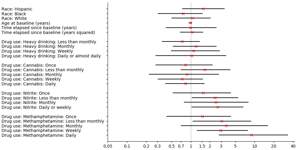
- Heavy drinking: Effects cluster around 1. What trend exists between amount of drinking and risky sex is negative. The CIs mostly overlap.
- Cannabis: Rare use seems associated with slightly more risky sex than no use, whereas the other usage levels are similar to each other and associated with slightly less.
- Alkyl nitrites: Effects point towards alkyl nitrite use being associated with more risky sex, but the effects of frequencies beyond "Once" are all similar (an odds ratio around 2.5).
- Methamphetamine: "Once" is associated with slight risk; "Rarely", "Montly", and "Weekly" with greater risk; "Daily" with major risk.
(rd 2 (digest-indicator (go-indicator
  d "HIV+" "risky_sex_transmit_d" "Risky")))
| I | point | lo | hi |
|---|---|---|---|
| (Intercept) | 0.37 | 0.07 | 2.14 |
| race_hispanic: TRUE | 0.87 | 0.42 | 1.72 |
| race_black: TRUE | 1.13 | 0.49 | 2.66 |
| race_white: TRUE | 1.13 | 0.65 | 1.94 |
| age_at_baseline | 0.99 | 0.95 | 1.03 |
| years_since_baseline | 0.86 | 0.37 | 2.15 |
| years2_since_baseline | 1.02 | 0.62 | 1.48 |
| drug_sr_alcohol_heavy: Less than monthly | 0.77 | 0.42 | 1.34 |
| drug_sr_alcohol_heavy: Monthly | 1.32 | 0.60 | 2.76 |
| drug_sr_alcohol_heavy: Weekly | 0.98 | 0.40 | 2.07 |
| drug_sr_alcohol_heavy: Daily or almost daily | 0.97 | 0.19 | 3.02 |
| drug_sr_cannabis: Once | 0.83 | 0.22 | 2.36 |
| drug_sr_cannabis: Rarely | 1.06 | 0.40 | 2.37 |
| drug_sr_cannabis: Monthly | 0.51 | 0.13 | 1.42 |
| drug_sr_cannabis: Weekly | 0.96 | 0.37 | 2.10 |
| drug_sr_cannabis: Daily | 0.65 | 0.33 | 1.18 |
| drug_sr_alkyl_nitrite: Once | 0.36 | 0.06 | 1.06 |
| drug_sr_alkyl_nitrite: Rarely | 1.98 | 1.01 | 4.24 |
| drug_sr_alkyl_nitrite: Monthly | 0.66 | 0.19 | 1.58 |
| drug_sr_alkyl_nitrite: Daily or weekly | 1.63 | 0.84 | 3.45 |
| drug_sr_meth: Once | 1.20 | 0.46 | 2.86 |
| drug_sr_meth: Rarely | 1.44 | 0.70 | 3.12 |
| drug_sr_meth: Monthly | 1.79 | 0.71 | 4.35 |
| drug_sr_meth: Weekly | 2.29 | 1.17 | 4.84 |
| drug_sr_meth: Daily | 2.27 | 1.12 | 5.06 |
(plot-indicator (go-indicator
  d "HIV+" "risky_sex_transmit_d" "Risky"))
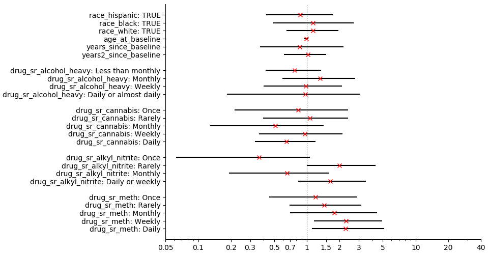
- Heavy drinking: Effects cluster around 1 and are not monotonic.
- Cannabis: Montly use seems associated with somewhat less risky sex than no use, whereas the other usage levels are around 1.
- Alkyl nitrites: A zig-zag trend. The biggest effect is that "Once" is associated with substantially lower risk, but note the very wide CI.
- Methamphetamine: A monotonic-looking positive effect that starts very weak at "Once" (OR 1.2) but becomes moderate at "Weekly" and "Daily" "Daily" (OR 2.3).
(rd 2 (digest-indicator (go-indicator
  d "HIV+" "hiv_load_detect" "Detectable")))
| I | point | lo | hi |
|---|---|---|---|
| (Intercept) | 0.37 | 0.04 | 3.61 |
| race_hispanic: TRUE | 1.30 | 0.48 | 3.94 |
| race_black: TRUE | 1.78 | 0.60 | 5.59 |
| race_white: TRUE | 1.04 | 0.45 | 2.29 |
| age_at_baseline | 1.04 | 0.99 | 1.09 |
| years_since_baseline | 0.56 | 0.22 | 1.33 |
| years2_since_baseline | 1.33 | 0.87 | 2.15 |
| drug_sr_alcohol_heavy: Less than monthly | 1.31 | 0.67 | 2.58 |
| drug_sr_alcohol_heavy: Monthly | 1.79 | 0.77 | 4.97 |
| drug_sr_alcohol_heavy: Weekly | 1.07 | 0.36 | 3.24 |
| drug_sr_alcohol_heavy: Daily or almost daily | 0.40 | 0.08 | 1.83 |
| drug_sr_cannabis: Once | 1.38 | 0.42 | 5.66 |
| drug_sr_cannabis: Rarely | 1.59 | 0.59 | 4.98 |
| drug_sr_cannabis: Monthly | 0.31 | 0.08 | 1.08 |
| drug_sr_cannabis: Weekly | 1.97 | 0.65 | 7.21 |
| drug_sr_cannabis: Daily | 1.22 | 0.55 | 2.78 |
| drug_sr_alkyl_nitrite: Once | 0.42 | 0.14 | 1.13 |
| drug_sr_alkyl_nitrite: Rarely | 0.85 | 0.38 | 1.93 |
| drug_sr_alkyl_nitrite: Monthly | 0.48 | 0.15 | 1.41 |
| drug_sr_alkyl_nitrite: Daily or weekly | 1.38 | 0.52 | 3.96 |
| drug_sr_meth: Once | 0.76 | 0.28 | 2.22 |
| drug_sr_meth: Rarely | 1.02 | 0.41 | 2.63 |
| drug_sr_meth: Monthly | 2.41 | 0.97 | 8.63 |
| drug_sr_meth: Weekly | 2.64 | 1.22 | 6.95 |
| drug_sr_meth: Daily | 3.33 | 1.34 | 9.67 |
(plot-indicator (go-indicator
  d "HIV+" "hiv_load_detect" "Detectable"))
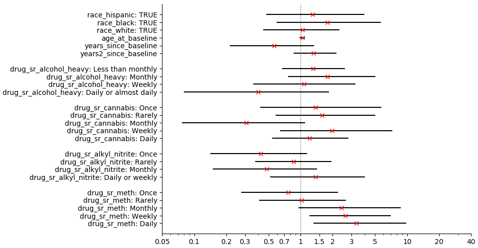
- Heavy drinking: Effects range from slightly positive ("Monthly", OR 1.8) to substantially negative ("Daily or almost daily", OR 0.4).
- Cannabis: No clear trend. Monthly use is associated with substantially lower risk of having a detectable viral load (OR 0.3). Weekly, with moderately higher risk (OR 2.0).
- Alkyl nitrites: A zig-zag. The biggest effect is "Once", which is associated with moderately lower risk.
- Methamphetamine: A monotonic-looking trend from "Once" (OR 0.8) to "Daily" (OR 3.3).