Rickrack notebook

Created 2 Nov 2013 • Last modified 7 Jul 2015

MTurk study

Goal

To establish the test–retest (and, when possible, parallel-forms) reliability and the criterion validity of econometric tests, particularly tests of patience, stationarity, risk aversion, and loss aversion. Well, maybe including all four would be biting off more than I'd care to chew, but I am at least interested in the first two. Brass and Hazel need reliable tests, particularly so that negative results can be interpretable.

A reasonable way to assess reliability under my predictivist philosophy is just to try to predict scores with themselves.

Basic plan

Use Tversky so both MTurk and the lab are usable
Administer tests twice at time A and only once at time B; use the difference between the first two for parallel-forms reliability and the difference between A and B for test-retest reliability (possibly intermingled with parallel-forms, of course)
Also measure criterion variables at time A (criterion variables are important if only so we have a way to compare tests that use model-heavy and model-light techniques, and therefore broader and narrower operationalizations of the construct being measured)

Finally, Christian points out that it would be nice to demonstrate that patience in immediate-versus-delayed dilemmas is less stable over time than patience in delayed-versus-delayed. The theory of construal level and psychological distance predicts that one should adopt a more concrete mindset in immediate-versus-delayed situations. Perhaps this more concrete mindset would lead to preferences that are more influenced by short-term concerns and therefore less stable over time. Then again, you wouldn't need such fancy concepts as construal level and psychological difference to explain this: people should indeed be more influenced by present circumstances when making a decision involving the present.

Previous work

(What tests already exist? What reliabilities and validities have been demonstrated for exactly which tests?)

Going by Schuerger, Tait, and Tavernelli (1982), personality tests have reliability coefficients of roughly .8 for 1–2 weeks and .6 for 1 year.

Intertemporal choice
- Reliability (how exhaustive can this be made?)
  - Kirby, Petry, and Bickel (1999): Used a relatively coarse 7-trial forced-choice patience test for each of three reward magnitudes, yielding three ln(k)s. Immediate SSes only. Heroin addicts had higher ln(k)s (i.e., were less patient) than controls (but the analysis seems to have ignored the triplet grouping of the ln(k)s). Correlation of the ln(k)s with intelligence (as measured by the WAIS) was small.
  - Kirby (2009): Used the same patience test as Kirby et al. (1999). The reliability correlation of mean ln(k) (mean across the three reward magnitudes) was .77 (95% CI [.67, .85]) for 5 weeks and .71 ([.5, .84]) for 1 year.
  - Beck and Triplett (2009): Subjects selected from a list the immediate equivalent to $1,000 at six different delays. Then hyperbolic ks were (somehow) fit. For the 85% of subjects who discounted in an orderly fashion, ln(k) correlated .64 over a 6-week interval.
  - Smith and Hantula (2008): A forced-choice patience test and a free-response patience test yielded ks correlated at .75, but AUCs correlated at .33.
- Validity (we will of course cite only examples)
  - Madden, Petry, Badger, and Bickel (1997): A stepwise procedure finding x such that $x immediately is equivalent to $1,000 at each of six delays. Then a hyperbolic function was fit by least squares and the k extracted. Heroin addicts had higher ks than controls. ks correlated .4 with scores on the Impulsivity subscale of the Eysenck Personality Questionnaire.
  - Sutter, Kochaer, Rützler, and Trautmann (2010): A paper-and-pencil faux-stepwise procedure with several different delay and amount conditions, including non-immediate SSDs. Variables concerning drug use, BMI, saving, and grades are included, but the numerical results are a bit hard to digest.
  - Chabris, Laibson, Morris, Schuldt, and Taubinsky (2008): Used Kirby et al.'s (1999) patience-test items, but estimated discounting rate using the MLE of a parameter in a logistic model. Correlations with various individual "field behaviors" are low, and with aggregate indices of field behaviors range from .09 to .38.
  - Wulfert, Block, Ana, Rodriguez, and Colsman (2002): A single real choice between $7 today and $10 in a week. Choice was correlated in the expected directions with being a problem student, GPA, and drug use from .52 to .68.
Loss aversion
- Existing loss-aversion test: coin-toss paradigm; Harinck, Van Dijk, Van Beest, & Mersmann, 2007, observes that for small gains, people are willing to write loss amounts implying negative EV
Risk aversion
- Weber and Chapman (2005) found that people will take riskier gambles with smaller amounts of money (the "peanuts effect")

One would like tests that are repeatable (i.e., tests that can be re-administered very soon after; i.e., tests for which remembering one's past answers is not a problem), so they can be used as state measures. Possibly many existing tests meet this criterion despite using a fixed item set, since giving people the same item twice in past intertemporal-choice studies has frequently revealed them to not be perfectly consistent.

One can use already existing patience tests, particularly that of Kirby et al. (1999). The reliability correlations, although less than one might want, don't have much room for improvement, after all. However, this test doesn't measure stationarity, it doesn't consider nonzero SSDs, it's coarse, and it's questionably repeatable. These qualities may or may not be bad. They might end up making the test better at predicting theoretically patience-relevant criterion variables. But that's an empirical question, and you certainly wouldn't these qualities a priori. So let's at least consider some other tests.

Theory and nonzero SSDs

Can the idea of temporal discounting accommodate nonstationarity in the wrong direction (i.e., becoming more patient as front-end delays increase)? I think it must. A test of stationarity is then a test of "relative future patience", or inversely "immediacy bias", which can rate subjects as nonstationarity in the classical direction, nonstationary in the wrong direction, or perfectly stationary.

The distinction between immediate–delayed versus delayed–delayed choices can be thought of like this:

Immediate vs. delayed: choices under the gun
Delayed vs. delayed: plans for the future

It looks like I'm going to measure nonstationarity using two discount factors, one immediate-versus-delayed and one delayed-versus-delayed. How should it be computed? Let's say as the difference. Then if I want to include both patience and nonstationarity as predictors in a regression model, I can just include one term for each discount factor: the model μ = b₀ + b₁ID + b₂DD is just a reparametrization of μ = b₀ + b₁ID + b₂(DD − ID). Since I don't believe in interpreting model parameters, the difference between these models is immaterial.

Can we use established techniques of CAT?

(Short answer: apparently not if we want our tests to be easy to implement and require low resources.)

Okay, suppose we want to use the minimum expected posterior variance criterion (equation 1.26 of van der Linden & Glas, 2010), and we're using a one-parameter binary-choice model. Then for each round we need to find a new item Y minimizing

p(Y = 1 | x) * Var(θ | x, Y = 1) +  p(Y = 0 | x) * Var(θ | x, Y = 0)

where x is the data already obtained. Let us suppose our model is

Y ~ Bern(ilogit(ρ (v_{30} * lr - sr)))

and we're using some fixed value of ρ instead of treating it as a free parameter. Rename v₃₀ to θ. If we use a uniform prior for θ, the posterior is proportional to the likelihood.

In the case of multiple trials, just take the log of each and sum them all up, then exponentiate.

I don't think there are closed forms for p(Y = 1 | x) and Var(θ | x, Y = 1), because there's no conjugate prior for θ. And for a uniform prior, it doesn't seem like a closed form for the mean exists once we have data from more than one trial.

Moreover, grid sampling alone doesn't seem like it can help, because we would need to do a full grid sample or three for every candidate Y.

Tests

(Christian suggests it would be interesting to compare actual discount factors between the tests.)

Intertemporal choice
- 20 rounds of probabilistic bisection search (Horstein, 1963; Waeber, 2013, p. 14) with p_c = .75. What is being searched for is the one-month discount factor, so each trial is a forced choice between an immediate reward and a 30-day-delayed reward. The ratio between these rewards is what is manipulated adaptively; the absolute amounts can be varied more or less arbitrarily.
- Bisection search again, but with a one-month front-end delay added to both delays.
- A non-adaptive free-response task, where the subject types in an indifference amount (for immediate versus month-delayed). Mike Bixter says subjects find filling in the LLR easier, but beware that (going by the results of Builder) Turkers tend to be patient. The fixed amount can be determined randomly, and the discount factor can be estimated as the mean of the ratios.
- Free-response again, but with a one-month front-end delay.
- The test of Kirby (2009) (plus front-end delays?)
Criterion (partly from Chabris et al., 2008) - see the source code for details

TV 1, 2

I've done a bit of a trial run with just bisection search.

rd(transform(
    dcast(
        ss(itb.discs, sb[char(s), "tv"] %in% 1:2),
        s + type ~ round,
        value.var = "disc"),
    change = round2 - round1))

	s	type	round1	round2	change
1	s0001	near	0.651	0.597	-0.053
2	s0001	far	0.599	0.518	-0.081
3	s0003	near	0.292	0.622	0.330
4	s0003	far	0.712	0.789	0.077
5	s0004	near	0.994	0.994	0.000
6	s0004	far	0.994	0.994	0.000
7	s0005	near	0.867	0.916	0.049
8	s0005	far	0.868	0.783	-0.085
9	s0006	near	0.752	0.766	0.015
10	s0006	far	0.745	0.618	-0.127
11	s0007	near	0.292	0.440	0.148
12	s0007	far	0.556	0.442	-0.113
13	s0008	near	0.844	0.974	0.131
14	s0008	far	0.982	0.980	-0.002
15	s0010	near	0.959	0.994	0.034
16	s0010	far	0.981	0.994	0.013
17	s0012	near	0.994	0.994	0.000
18	s0012	far	0.994	0.994	0.000
19	s0013	near	0.500	0.534	0.034
20	s0013	far	0.594	0.525	-0.068
21	s0014	near	0.810	0.908	0.098
22	s0014	far	0.879	0.890	0.011
23	s0016	near	0.625	0.615	-0.010
24	s0016	far	0.519	0.509	-0.010
25	s0017	near	0.796	0.880	0.084
26	s0017	far	0.835	0.799	-0.036
27	s0018	near	0.672	0.597	-0.075
28	s0018	far	0.738	0.578	-0.160

near is immediate versus 1 month, and far is 1 month versus 2 months. round1 and round2 are the discount factors resulting from the first and second rounds (respectively) of the given test.

The discount factors themselves generally look okay, except for those annoying subjects who chose LL every time. Let's graph the changes from time 1 to time 2.

discs.tv2 = ss(itb.discs,
    sb[char(s), "tv"] %in% 1:2 &
    sb[char(s), "itb.caught.s1"] == 0 &
    sb[char(s), "itb.ll.s1"] < 1)

dodge(type, round2 - round1, data = dcast(
    discs.tv2,
    s + type ~ round,
    value.var = "disc")) + boxp

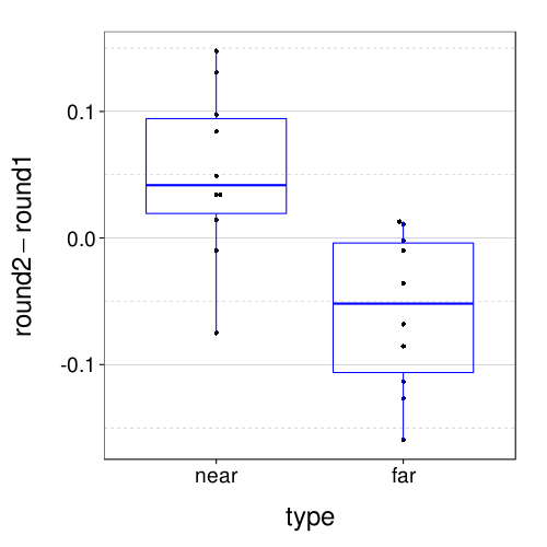
rd(with(dcast(discs.tv2, s + type ~ round, value.var = "disc"),
    qmean(abs(round2 - round1))))

	value
lo	0.006
mean	0.065
hi	0.154

Looks like there's a trend for scores on the two tests to drift in opposite directions. Rummy, but I have a small sample, anyway. More important is to note that changes in the discount factor generally don't exceed .1. That's good.

How do discount factors (and changes in discount factors) change if we use only 10 (non-catch) trials per round? Can we safely use just 10 trials?

rd(with(
    ss(merge(itb.discs, itb.discs10, by = qw(s, type, round)),
        sb[char(s), "tv"] %in% 1:2 &
        sb[char(s), "itb.caught"] == 0 &
        sb[char(s), "itb.ll"] < 1),
    qmean(abs(disc.x - disc.y))))

	value
lo	0.002
mean	0.051
hi	0.140

.05 units seems like too large an increase in error to accept, since it's on the order of the immediate-retest error for the full, 20-trial estimate.

Notice that the median of obtained discounts is about .75:

dodge(type, disc, data = discs.tv2) + boxp +
    coord_cartesian(ylim = c(0, 1.05))

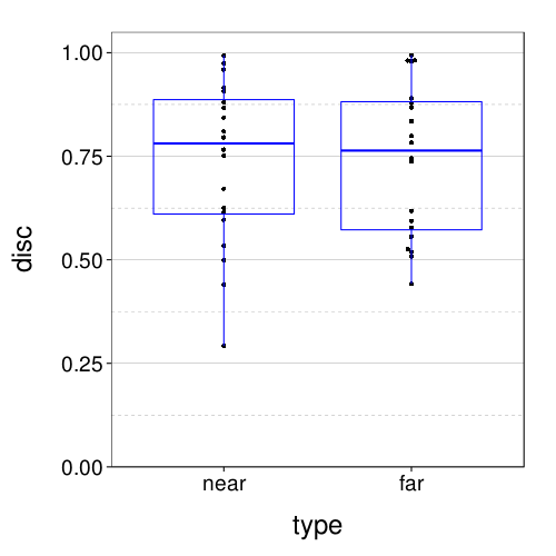
So, I might as well set the prior density in the bisection test to have median .75 instead of .5. For simplicity, it can remain uniform on either side of .75.

Here are the criterion variables:

ss(sb, tv %in% 1:2)[criterion.vs]

	bmi	tobacco	cigpacks	gambling	exercise	healthy.meals	floss	cc.latefees	cc.subpay	savings
s0001	22.95737	TRUE	1	2	10	0.60	0	0	0.75	0.05
s0003	24.03070	FALSE		2	25	0.70	7	0	0.12	0.10
s0004	27.89405	FALSE		0	20	0.75	0	0	0.00	0.20
s0005	26.13806	FALSE		0	16	0.90	0	0	0.00	0.05
s0006	19.34512	FALSE		0	9	0.70	2	1	0.01	0.00
s0007	27.97930	FALSE		0	8	0.70	4	0	0.00	0.00
s0008	24.37399	FALSE		0	70	0.90	3	3	1.00	0.00
s0010	24.10524	FALSE		0	15	0.95	7	0	0.00	0.30
s0012	23.40337	FALSE		0	8	0.90	9	0	0.00	0.80
s0013	20.94104	TRUE	7	0	10	0.10	0	0	0.48	0.00
s0014	27.12460	FALSE		0	5	0.80	3	0	0.50	0.20
s0016	18.98722	FALSE		0	0	0.10	0	0	0.99	0.00
s0017	24.67918	FALSE		0	5	0.05	0	1	0.00	0.20
s0018	28.40975	TRUE	1	1	3	0.90	0	0	0.24	0.05

TV 3, 4

This time I used just free-response matching.

rd(transform(
    dcast(
        ss(itm.discs, sb[char(s), "tv"] %in% 3:4),
        s + type ~ round,
        value.var = "disc"),
    change = round2 - round1))

	s	type	round1	round2	change
1	s0020	near	0.673	0.692	0.018
2	s0020	far	0.738	0.655	-0.082
3	s0021	near	0.033	0.033	0.000
4	s0021	far	0.500	0.500	0.000
5	s0022	near	0.831	0.837	0.006
6	s0022	far	0.829	0.811	-0.019
7	s0023	near	0.913	0.921	0.007
8	s0023	far	0.908	0.894	-0.015
9	s0024	near	0.546	0.558	0.011
10	s0024	far	0.569	0.465	-0.105
11	s0025	near	0.913	0.861	-0.052
12	s0025	far	0.903	0.836	-0.067
13	s0026	near	0.843	0.910	0.067
14	s0026	far	1.000	1.000	0.000
15	s0028	near	0.815	0.859	0.044
16	s0028	far	0.908	0.733	-0.174
17	s0029	near	0.597	0.669	0.072
18	s0029	far	0.333	0.541	0.208
19	s0030	near	0.809	0.776	-0.033
20	s0030	far	0.859	0.800	-0.059
21	s0031	near	0.450	0.463	0.013
22	s0031	far	0.488	0.472	-0.016
23	s0032	near	0.500	0.505	0.005
24	s0032	far	0.500	0.504	0.004
25	s0034	near	0.262	0.411	0.149
26	s0034	far	0.466	0.437	-0.029
27	s0035	near	0.357	0.273	-0.084
28	s0035	far	0.187	0.227	0.040

discs.tv4 = ss(itm.discs,
    sb[char(s), "tv"] %in% 3:4 &
    sb[char(s), "itm.backwards.s1"] == 0)

dodge(type, round2 - round1, data = dcast(
    discs.tv4,
    s + type ~ round,
    value.var = "disc")) + boxp

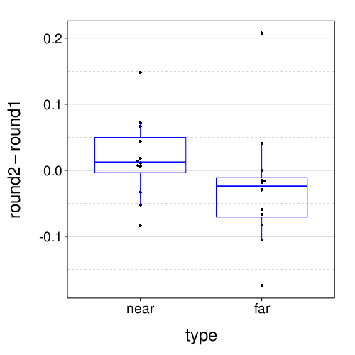
rd(with(dcast(discs.tv4, s + type ~ round, value.var = "disc"),
    qmean(abs(round2 - round1))))

	value
lo	0.004
mean	0.057
hi	0.188

The opposite-direction drift pattern shows up again, but now the error is, if anything, smaller. Nice.

Again, let's ask how estimates would change if we halved the number of trials.

rd(with(
    ss(merge(itm.discs, itm.discs5, by = qw(s, type, round)),
        sb[char(s), "tv"] %in% 3:4 &
        sb[char(s), "itm.backwards.s1"] == 0),
    qmean(abs(disc.x - disc.y))))

	value
lo	0.000
mean	0.019
hi	0.060

That's actually not a bad increase in error considering how quick the test becomes if it's shortened to 5 trials. What about if we use only the first trial?

rd(with(
    ss(merge(itm.discs, ss(itm, tn == 1), by = qw(s, type, round)),
        sb[char(s), "tv"] %in% 3:4 &
        sb[char(s), "itm.backwards.s1"] == 0),
    qmean(abs(ssr/equiv - disc))))

	value
lo	0.000
mean	0.067
hi	0.299

Yeah, I didn't think that would work as well. Now let's look at the retest errors for the 5-trial version.

dodge(type, round2 - round1, data = dcast(
    ss(itm.discs5,
        sb[char(s), "tv"] %in% 3:4 &
        sb[char(s), "itm.backwards.s1"] == 0),
    s + type ~ round,
    value.var = "disc")) + boxp

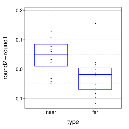
rd(with(
    dcast(
        ss(itm.discs5, sb[char(s), "tv"] %in% 3:4 & sb[char(s), "itm.backwards.s1"] == 0),
        s + type ~ round,
        value.var = "disc"),
    qmean(abs(round2 - round1))))

	value
lo	0.008
mean	0.063
hi	0.172

Not as good, but it's hard to say how much worse, or if the difference is meaningful. It isn't obviously better or worse than fig--g/tv2-itb-retest-diffs.

dodge(type, disc, data = discs.tv4) + boxp +
    coord_cartesian(ylim = c(0, 1.05))

Very similar to last time, with perhaps a bit more variability.

Planning for the real thing

There are six intertemporal-choice tests, namely, one immediate–delayed version and one delayed–delayed version of bisection, matching, and Kirby-style fixed forced-choice.

This last kind of test, which I haven't tried out yet, may as well use the medium reward size (since this is perhaps the most reliable, going by table 2 of Kirby, 2009). The front-end delay we add could be 30 days for consistency with the other tests.

Session 1
- The intertemporal-choice tests, in random order
- Again, also in random order
- Criterion tests
Session 2
- The intertemporal-choice tests, in random order

A reasonable retest interval would be 5 weeks, but should we pay any heed to the relationship between the retest interval and the front-end delays?

(Which session-1 tests predict session-2 near better, near or far? It's probably better for the interval to be bigger than the front-end delay than smaller.)

Administering the intertemporal tests only once in session 1 would be one way to keep costs down.

Scoring the fixed-quartet test

How shall we score this test? At least trying to imitate Kirby's (2009) method as closely as possible probably makes sense to do at some point, but it is not necessarily the best choice of scoring procedure. In particular, I would like a scoring procedure that is unaffected by front-end delay, for easier comparison between near and far conditions, whereas Kirby (2009) uses hyperbolic discount rates.

The Kirby items are deliberately designed such that the logarithms of their hyperbolic discount rates of indifference are about equally spaced. This seems to also be the case for exponential discount rates:

kirby = data.frame(
    ssr = c(54, 47, 54, 49, 40, 34, 27, 25, 20),
    llr = c(55, 50, 60, 60, 55, 50, 50, 60, 55),
    delay = c(117, 160, 111, 89, 62, 30, 21, 14, 7))
rd(diff(with(kirby,
    log( (log(llr) - log(ssr)) / (delay - 0) ))))

	value
	0.903 0.898 0.874 0.814 0.917 0.825 0.757 0.838

However, I really don't want to be seen as taking a side on the exponential–hyperbolic debate here. And besides, if the spacing is uniform, it stands to reason that scoring with log discount rates should be about equivalent to scoring with the "rank" of the item (1, 2, etc.), which is a lot simpler. So let's do that.

For consistency with Kirby, we'll assign to each subject their most consistent rank, resolving ties by averaging all consistent ranks (using an arithmetic mean in our case since we aren't following this up with logarithms). To ensure that most scores are integers on the scale of 0 to 20, we'll also double them and subtract 2.

Single-test analyses

Current sample size:

c("All subjects" = sum(with(sb, tv %in% 5:8)),
    "Included subjects only" = sum(with(sb, tv %in% 5:8 & good)))

	value
All subjects	200
Included subjects only	181

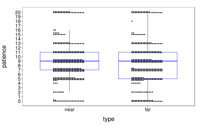
Fixed quartets

Here all the scores in the near and far conditions (with two data points per subject, one for each round):

dodge(type, patience, discrete = T, stack.width = 20,
    data = ss(itf.scores, sb[char(s), "tv"] %in% 5:8 & s %in% good.s)) + boxp

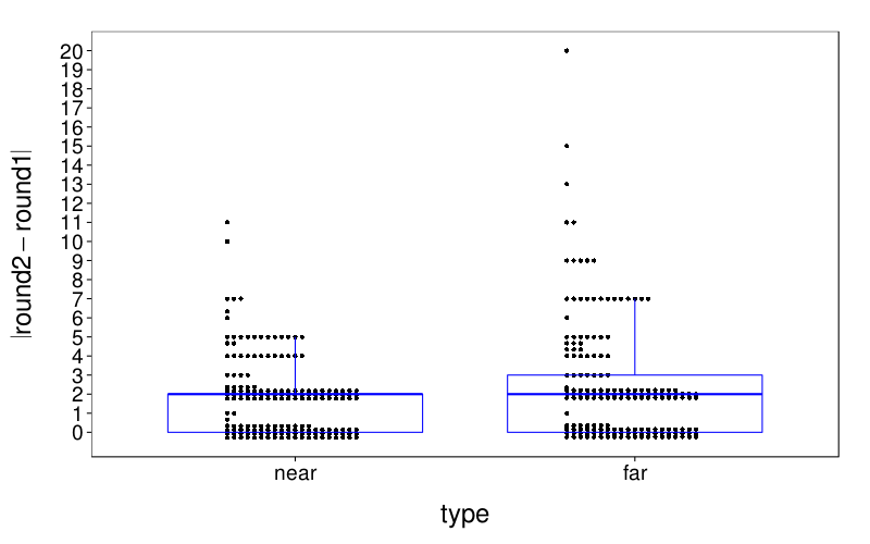
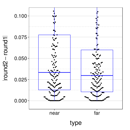
Here are the absolute retest differences in the near and far conditions:

dodge(type, abs(round2 - round1), discrete = T, stack.width = 20, data = dcast(
    ss(itf.scores, sb[char(s), "tv"] %in% 5:8 & s %in% good.s),
    s + type ~ round,
    value.var = "patience")) + boxp

Here are test–retest correlations:

d = dcast(ss(itf.scores, sb[char(s), "tv"] %in% 5:8 & s %in% good.s),
    s ~ type + round, value.var = "patience")
rd(d = 2, data.frame(
   row.names = qw(near, far),
   pearson = c(cor(d$near_round1, d$near_round2, method = "pearson"),
       cor(d$far_round1, d$far_round2, method = "pearson")),
   spearman = c(cor(d$near_round1, d$near_round2, method = "spearman"),
       cor(d$far_round1, d$far_round2, method = "spearman"))))

	pearson	spearman
near	0.85	0.81
far	0.72	0.71

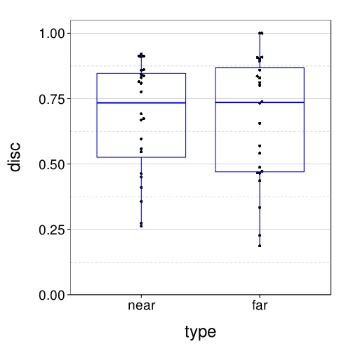
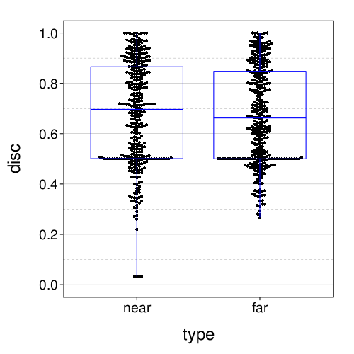
Bisection

Here all the scores in the near and far conditions (with two data points per subject, one for each round):

dodge(type, disc,
        data = ss(itb.discs, sb[char(s), "tv"] %in% 5:8 & s %in% good.s)) +
    scale_y_continuous(breaks = seq(0, 1, .2)) +
    coord_cartesian(ylim = c(-.05, 1.05)) +
    boxp

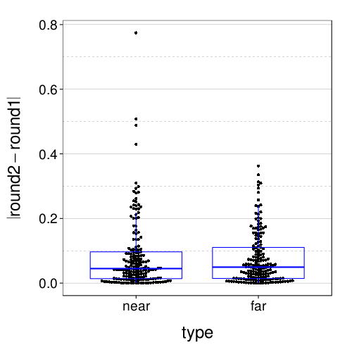
Here are the absolute retest differences in the near and far conditions:

fig = dodge(type, abs(round2 - round1), data = dcast(
    ss(itb.discs, sb[char(s), "tv"] %in% 5:8 & s %in% good.s),
    s + type ~ round,
    value.var = "disc")) + boxp
fig

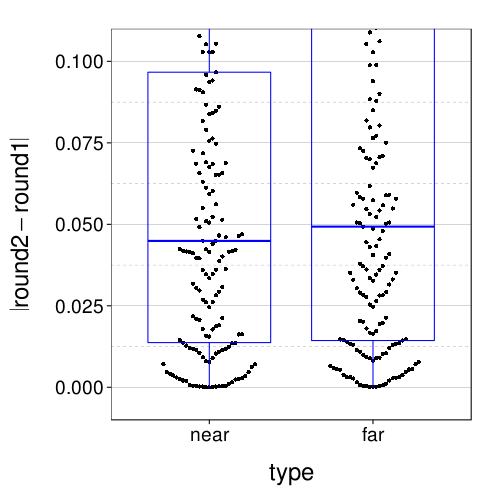
Let's zoom in:

fig + coord_cartesian(ylim = c(-.01, .11))

Here are test–retest correlations:

d = dcast(ss(itb.discs, sb[char(s), "tv"] %in% 5:8 & s %in% good.s),
    s ~ type + round, value.var = "disc")
rd(d = 2, data.frame(
   row.names = qw(near, far),
   pearson = c(cor(d$near_round1, d$near_round2, method = "pearson"),
       cor(d$far_round1, d$far_round2, method = "pearson")),
   spearman = c(cor(d$near_round1, d$near_round2, method = "spearman"),
       cor(d$far_round1, d$far_round2, method = "spearman"))))

	pearson	spearman
near	0.76	0.80
far	0.81	0.81

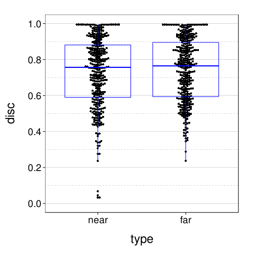
Matching

Here all the scores in the near and far conditions (with two data points per subject, one for each round):

dodge(type, disc,
    data = ss(itm.discs, sb[char(s), "tv"] %in% 5:8 & s %in% good.s)) +
    scale_y_continuous(breaks = seq(0, 1, .2)) +
    coord_cartesian(ylim = c(-.05, 1.05)) +
    boxp

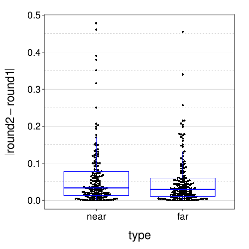
Here are the absolute retest differences in the near and far conditions:

fig = dodge(type, abs(round2 - round1), data = dcast(
    ss(itm.discs, sb[char(s), "tv"] %in% 5:8 & s %in% good.s),
    s + type ~ round,
    value.var = "disc")) + boxp
fig

Let's zoom in:

fig + coord_cartesian(ylim = c(-.01, .11))

Here are test–retest correlations:

d = dcast(ss(itm.discs, sb[char(s), "tv"] %in% 5:8 & s %in% good.s),
    s ~ type + round, value.var = "disc")
rd(d = 2, data.frame(
   row.names = qw(near, far),
   pearson = c(cor(d$near_round1, d$near_round2, method = "pearson"),
       cor(d$far_round1, d$far_round2, method = "pearson")),
   spearman = c(cor(d$near_round1, d$near_round2, method = "spearman"),
       cor(d$far_round1, d$far_round2, method = "spearman"))))

	pearson	spearman
near	0.88	0.89
far	0.91	0.91

Criterion variables

transform(ss(sb, tv %in% 5:8 & good)[c("height.raw", "weight.raw", criterion.vs)],
    bmi = round(bmi))

	height.raw	weight.raw	bmi	tobacco	cigpacks	gambling	exercise	healthy.meals	floss	cc.latefees	cc.subpay	savings
s0038			27	FALSE		0	14	1.00	14			0.00
s0042			22	FALSE		0	20	0.50	0	0	0.01	0.00
s0046			26	FALSE		0	8	0.90	0	0	1.00	0.30
s0051			42	FALSE		0	3	0.25	0	0	0.00	0.00
s0052			32	FALSE		0	4	0.02	7	2	0.01	0.20
s0053			24	FALSE		0	10	0.00	7	0	0.00	0.00
s0055			21	FALSE		0	2	0.75	14	0	0.40	0.20
s0056			25	FALSE		0	10	0.85	0	0	0.00	0.00
s0059			35	FALSE		1	3	0.75	0			0.06
s0062			20	FALSE		0	14	0.60	7	0	0.00	0.10
s0064			23	FALSE		3	10	0.67	7	0	0.00	0.10
s0066			23	FALSE		0	5	0.85	7	0	0.00	0.20
s0067			30	FALSE		0	10	0.75	7	0	0.00	0.35
s0068			22	FALSE		0	0	0.00	0	0	0.00	0.20
s0070			25	FALSE		0	7	0.80	0	0	0.00	0.30
s0078			30	FALSE		1	0	0.00	0	0	0.80	0.00
s0080			37	FALSE		0	10	0.25	5	0	0.40	0.05
s0082			24	FALSE		0	15	0.67	2	3	0.90	0.10
s0083			32	FALSE		0	25	0.10	7			0.01
s0084			23	FALSE		0	10	0.05	0			0.00
s0085	69in	147lbs	22	FALSE		2	2	0.75	4			0.40
s0087	5ft	105 pounds	21	TRUE	2	1	12	1.00	4			0.01
s0088	5 ft 5 in	140 pounds	23	FALSE		4	6	0.50	3	2	0.02	0.50
s0091	6 ft 5 in	170 pounds	20	FALSE		0	12	0.00	5	1	0.22	0.15
s0092	6 ft 1 in	150 pounds	20	FALSE		0	10	0.25	0	3	1.00	0.00
s0095	5 ft 6 in	115 pounds	19	FALSE		0	5	0.80	6	0	0.03	0.15
s0096	5 ft 11 in	180 pounds	25	FALSE		4	3	0.60	0	0	0.25	0.10
s0099	5 ft 5 in	190 pounds	32	FALSE		0	5	0.80	12	0	0.90	0.10
s0100	5 ft 6 in	133 pounds	21	FALSE		0	0	0.50	1	0	0.00	0.10
s0104	6 ft 0 in	207 pounds	28	FALSE		0	3	0.60	0	0	0.90	0.00
s0106	5 ft 1 in	150 pounds	28	FALSE		0	3	1.00	7	0	1.00	0.05
s0107	5 ft 10 in	200 pounds	29	FALSE		0	3	1.00	7	2	1.00	0.30
s0108	5 ft 11 in	155 pounds	22	TRUE	7	0	21	1.00	14	0	0.00	0.63
s0111	5 ft 6 in	120 lb	19	FALSE		0	3	1.00	7	0	0.00	0.15
s0113	6 ft	210 pounds	28	TRUE	2	0	10	0.30	21			0.00
s0116	6 ft 1 in	170 pounds	22	FALSE		2	4	0.02	1	0	0.00	0.15
s0117	5 ft 8 in	155 pounds	24	FALSE		0	5	0.80	4	0	0.00	1.00
s0118	5 ft 9 in	176 pounds	26	FALSE		0	10	0.00	4			0.00
s0119	5 ft 5 in	130 pounds	22	TRUE	6	7	5	0.25	7	0	0.00	0.10
s0120	6ft 2 in	205 pounds	26	FALSE		0	3	0.03	3			0.10
s0121	5 ft 10 in	172 pounds	25	TRUE	7	0	15	0.85	7	0	0.00	0.15
s0123	5 ft 10 in	190 pounds	27	FALSE		0	4	0.02	7	0	0.05	0.15
s0124	5 ft 6 in	160 pounds	26	TRUE	4	0	16	0.80	7			0.00
s0125	5 ft 8 in	160 pounds	24	FALSE		0	1	0.00	1	0	0.20	0.10
s0126	5 ft 2 in	250 pounds	46	FALSE		0	1	0.00	0	0	0.75	0.05
s0127	5 ft 3 in	230 pounds	41	TRUE	7	0	4	0.35	0			0.09
s0128	5 ft 6 in	145 pounds	23	FALSE		0	0	0.40	0	0	0.00	0.20
s0129	5 ft 6 in	130 pounds	21	TRUE	7	0	4	0.90	7	0	0.00	0.10
s0132	5 ft 9 in	150 lbs	22	FALSE		0	1	0.90	0	10	0.99	0.00
s0135	6 ft 3 in	180 pounds	22	FALSE		0	6	0.50	0	0	0.25	0.10
s0137	5 ft 11 in	170 pounds	24	TRUE	3	0	2	0.00	0			0.00
s0138	6 ft 3 in	190 pounds	24	FALSE		0	4	0.25	7			0.00
s0139	6 ft 1 in	285 pounds	38	FALSE		0	10	0.50	5	0	0.90	0.00
s0140	5 ft 7 in	130 lbs	20	FALSE		0	5	0.20	1	3	0.50	0.23
s0141	5ft	92lbs	18	TRUE	1	0	20	0.80	0	1	0.60	0.10
s0142	5 Ft 10 IN	240lbs	34	FALSE		0	5	0.00	0			0.00
s0143	65in	165 pounds	27	FALSE		1	5	0.65	5			0.00
s0149	5ft 7in	140 pounds	22	TRUE	7	0	35	0.60	2	0	0.00	0.10
s0152	5 ft 5 in	135 pounds	22	FALSE		0	2	0.10	5			0.01
s0159	6ft	185 lbs	25	FALSE		0	10	0.95	5			0.00
s0167	5 ft 6in	135 lbs	22	FALSE		1	3	0.60	6	0	0.02	0.60
s0185	5 ft 6 in	140 pounds	23	TRUE	2	0	1	0.90	7			0.60
s0192	5 ft 8 in	145 pounds	22	FALSE		0	6	0.85	7	0	0.50	0.25
s0195	5 ft 10 in	168 pounds	24	FALSE		0	6	0.50	2	0	0.00	0.25
s0196	68 inches	135 pounds	21	FALSE		0	5	1.00	7	0	0.02	0.20
s0198	6 ft 4 in	170 lb	21	FALSE		0	15	0.01	14			0.25
s0199	5 ft 9 in	150 pounds	22	FALSE		30	3	0.70	7			0.25
s0204	5 ft 2 in	145 pounds	27	FALSE		0	0	0.50	0	3	1.00	0.05
s0205	72 in	178 pounds	24	FALSE		0	4	0.30	0	0	0.00	0.05
s0206	5ft8in	148 pounds	23	FALSE		0	2	0.75	2	0	1.00	0.10
s0207	5 ft 5 in	130 pounds	22	FALSE		0	2	0.25	7	0	1.00	0.05
s0208	6ft	165 pounds	22	TRUE	3	0	25	0.10	7	8	0.25	0.00
s0209	6 ft	140 pounds	19	FALSE		0	35	0.40	0			0.10
s0210	5 ft 4 in	207 pounds	36	FALSE		0	4	0.00	7	4	0.15	0.05
s0213	5 ft 6 in	133 pounds	21	FALSE		0	0	0.75	0			0.10
s0216	5 ft 11 in	200 pounds	28	TRUE	4	0	5	0.80	7			0.10
s0218	5 ft. 5 in	150 pounds	25	FALSE		0	3	0.50	14	0	0.00	0.10
s0220	5ft 11in	190 lb	26	FALSE		0	5	0.50	0			0.00
s0222	5 ft 9 in	180 lbs	27	TRUE	2	15	10	0.33	3	0	0.90	0.20
s0223	6 ft 1 in	200 lbs	26	FALSE		0	3	0.50	2			0.00
s0224	5.9 ft	203 pound	28	TRUE	3	0	2	0.00	7	0	0.00	0.10
s0225	5 ft 4 inches	148 lbs.	25	FALSE		0	4	0.90	3	2	1.00	0.06
s0227	5ft6in	130 pounds	21	FALSE		0	19	1.00	4	0	1.00	0.00
s0230	6 ft 2 in	190 pounds	24	TRUE	3	0	3	0.06	5	0	0.24	0.05
s0231	5 ft 10 in	205 pounds	29	FALSE		0	3	0.20	2	40	1.00	0.00
s0232	6ft 1inch	170 pounds	22	FALSE		0	5	0.75	0			0.05
s0234	5 ft 1 in	140 lbs	26	FALSE		0	3	0.50	7			0.00
s0235	5 ft 5 in	145 pounds	24	FALSE		0	5	0.50	7	2	1.00	0.00
s0237	5 ft 8 in	154 pounds	23	TRUE	3	1	6	0.07	0	0	0.00	0.20
s0238	6ft	190 pounds	26	FALSE		1	10	0.10	1	3	0.99	0.05
s0239	6ft 2in	190 pounds	24	FALSE		5	10	0.90	7	0	0.25	0.00
s0241	6 ft 0 in	295 pounds	40	FALSE		0	5	0.60	7	0	0.00	0.20
s0242	5 ft 4 in	128 pounds	22	FALSE		0	5	0.90	7	0	0.00	0.50
s0243	6 ft 2 in	205 pounds	26	FALSE		0	1	0.25	2	0	0.12	0.05
s0244	6ft	250 pounds	34	FALSE		0	10	1.00	7	0	0.00	0.00
s0245	5ft 6inches	180 pounds	29	TRUE	7	0	25	0.10	7			0.05
s0246	5 ft 7 in	132 pounds	21	FALSE		0	6	0.20	1			0.20
s0248	5 ft 4 in	112 pounds	19	FALSE		0	6	0.40	7	0	0.95	0.07
s0249	5 ft 7 in	132 pounds	21	TRUE	5	0	5	0.30	7	0	0.03	0.00
s0250	5 ft 9 in	165 pounds	24	FALSE		0	5	0.05	0	0	0.00	0.25
s0252	6ft 1in	173 pounds	23	FALSE		4	15	0.03	7	1	0.00	0.40
s0253	6 ft	175 pounds	24	TRUE	4	0	2	0.20	6	0	0.90	0.05
s0258	6 ft	230 pounds	31	FALSE		0	6	0.20	14	0	0.00	0.01
s0260	5ft 11in	170 pounds	24	FALSE		0	10	0.01	4			0.10
s0261	5ft 5in	101 pounds	17	FALSE		0	1	0.01	7	0	0.00	0.05
s0262	6 ft 0 in	165 pounds	22	TRUE	4	0	8	0.60	0	0	0.25	0.10
s0263	5 ft 2 in	122lbs	22	FALSE		0	5	0.65	7	0	0.00	0.10
s0264	6ft	157 pounds	21	FALSE		0	10	0.80	3	2	0.24	0.00
s0265	5 ft 7 in	200 lbs	31	FALSE		0	3	0.00	0	0	0.30	0.10
s0267	5 ft 5 in	115 pounds	19	FALSE		0	5	0.90	3	2	0.24	0.24
s0268	6 ft 2 in	185 pounds	24	FALSE		0	1	0.02	5	0	0.00	0.42
s0270	5 ft 11 in	230 pounds	32	FALSE		0	2	0.65	2	0	0.55	0.25
s0271	5 ft 11 in	165 pounds	23	FALSE		0	6	0.50	3	0	0.60	0.15
s0272	6 ft 2 in	223 lbs	29	TRUE	4	4	6	0.75	2	0	0.22	0.18
s0273	6ft0in	175 pounds	24	FALSE		0	10	0.00	0	5	0.10	0.00
s0274	6 ft 3 in	198 pounds	25	FALSE		0	5	0.65	0	0	0.95	0.06
s0275	5 ft 7 in	178 pounds	28	FALSE		0	30	0.40	0			0.90
s0276	5ft 4 in	170 pounds	29	TRUE	2	0	0	0.50	0			0.00
s0277	5 ft 7 in	170 pounds	27	TRUE	7	0	7	0.80	14	1	0.75	0.05
s0278	5 ft 1 in	127 pounds	24	FALSE		0	0	0.10	0	0	0.00	0.20
s0283	5 ft 4 in	190 pounds	33	FALSE		1	3	0.00	14	0	0.00	0.10
s0284	5 ft 4 in	166 pounds	28	TRUE	7	2	3	0.30	14	1	0.10	0.00
s0285	5 ft 4 in	138 pounds	24	FALSE		0	6	1.00	7			0.20
s0286	5ft 8in	150pounds	23	TRUE	7	0	40	0.75	15	0	0.12	0.10
s0287	5 ft 8 in	160 pounds	24	TRUE	7	0	5	0.80	7			0.30
s0289	6 ft 2 in	185 pounds	24	FALSE		0	4	0.15	5	2	0.15	0.08
s0290	5 ft 9 in	145 pounds	21	FALSE		0	5	0.60	7	0	0.00	0.15
s0292	5ft 9in	155 lbs	23	FALSE		1	7	0.50	10	0	0.80	0.05
s0294	5 ft 5 in	150 pounds	25	FALSE		0	3	0.10	5	1	0.12	0.10
s0295	5ft 10in	150 pounds	22	FALSE		5	6	0.80	5	1	0.00	0.15
s0299	5 ft 6 in	183 pounds	30	TRUE	2	0	7	0.00	7	12	0.20	0.00
s0300	6 ft 2 in	280 lbs	36	FALSE		0	12	0.75	24	0	1.00	0.20
s0301	5 ft 6 in	185 pounds	30	FALSE		0	14	0.50	5	0	0.00	0.00
s0302	5 ft 8 in	190 pounds	29	FALSE		0	1	0.60	1	0	0.50	0.00
s0304	5 ft 7 in	141 pounds	22	FALSE		0	5	0.70	0	0	0.00	0.30
s0305	6 ft	160 pounds	22	FALSE		0	7	0.50	3	0	0.00	0.00
s0307	6ft	170 pounds	23	TRUE	1	0	4	0.80	6	0	0.00	0.75
s0308	5 ft. 7 in.	165 pounds	26	FALSE		0	2	0.95	0	0	0.35	0.10
s0309	5 ft 8 in	355 pounds	54	FALSE		0	0	0.02	0	1	0.24	0.00
s0310	5 ft 4 in	150 lbs	26	TRUE	2	3	5	0.60	0	0	0.30	0.30
s0312	5 ft 4 in	175 pounds	30	TRUE	3	0	6	0.45	0	0	0.00	0.00
s0313	5 ft 11 in	190 pounds	26	TRUE	14	0	5	0.80	0	0	0.00	0.10
s0314	5 ft 4 in	136 pounds	23	FALSE		0	8	0.75	7			0.20
s0315	5 ft 6 in	200 pounds	32	TRUE	3	0	5	0.25	7	0	0.50	0.10
s0316	5ft 11in	195 pounds	27	FALSE		0	4	0.55	1	2	0.99	0.01
s0317	5 ft 5 in	155 pounds	26	TRUE	1	0	9	0.60	5	1	0.60	0.20
s0318	6ft 1in	215lb	28	FALSE		0	4	0.50	2	0	0.75	0.20
s0319	6 ft	170 pounds	23	TRUE	6	0	8	0.06	0			0.00
s0321	6 ft 3 in	230 pounds	29	FALSE		0	18	0.95	7			0.50
s0322	5 ft 7 in	130 pounds	20	TRUE	2	0	4	0.00	0			0.00
s0323	5 ft 11 in	160 pounds	22	FALSE		1	1	0.25	0	0	0.00	0.15
s0326	5 ft 7 in	137 pounds	21	FALSE		0	7	0.50	0			0.10
s0327	5 ft 10 in	181 pounds	26	TRUE	2	0	2	0.70	0			0.01
s0328	64 in	157 pounds	27	FALSE		0	4	0.25	3	3	0.95	0.00
s0329	5 ft 4 in	150 pounds	26	FALSE		0	12	0.80	1	6	0.75	0.05
s0331	6 ft 0 in	170 pounds	23	FALSE		0	10	0.80	2	0	0.25	0.05
s0334	5 ft 10 in	140 lbs	20	FALSE		0	7	0.00	0	0	0.00	0.00
s0335	5 ft 9 in	180 pounds	27	FALSE		0	5	0.00	7	0	0.24	0.15
s0337	5 ft 10 in	160 pounds	23	FALSE		0	5	0.80	2			0.10
s0338	6ft 3in	186 pounds	23	FALSE		0	0	0.75	7	0	0.00	0.15
s0340	6 ft 0 in	242 pounds	33	TRUE	7	2	0	0.03	0	0	0.24	0.10
s0341	5ft 4in	155 pounds	27	FALSE		0	5	0.85	2	5	0.90	0.10
s0342	6ft 1 in	200 pounds	26	FALSE		0	5	0.50	0	0	1.00	0.00
s0343	5 ft 11 in	180 pounds	25	TRUE	5	0	3	0.20	4	0	0.00	0.10
s0344	5 ft 8 in	170 pounds	26	FALSE		1	10	0.03	1			0.10
s0345	6 ft 5 in	270 pounds	32	TRUE	3	0	7	0.50	4	0	0.00	0.50
s0346	5 ft 8 in	135 pounds	21	FALSE		0	0	0.80	7			0.10
s0347	5 ft 11 in	135 pounds	19	FALSE		0	1	0.10	0	0	0.24	0.05
s0348	5 ft 6 in	128 pounds	21	FALSE		0	7	1.00	14	0	0.00	0.20
s0349	5 ft 4 in	105 pounds	18	FALSE		0	2	0.05	1	0	0.01	0.40
s0350	5 ft 8 in	145 pounds	22	FALSE		0	7	0.90	14	0	1.00	0.90
s0353	5ft 10in	205 pounds	29	FALSE		5	10	0.75	1	1	0.50	0.20
s0354	5 ft 0 in	100 pounds	20	TRUE	14	0	5	0.01	0			0.03
s0358	5 ft 11 in	230 pounds	32	FALSE		1	7	0.50	0	3	0.75	0.05
s0359	5 ft 11 in	160 pounds	22	TRUE	0	0	3	0.75	6			0.20
s0361	6 ft	150 pounds	20	FALSE		0	15	0.70	7	0	0.00	0.05
s0362	5 ft 3 in	135 pounds	24	TRUE	2	5	35	0.85	7			0.01
s0363	6 ft 2 in	230 pounds	30	FALSE		15	1	0.00	4	0	0.00	0.00
s0364	6 ft 1 in	230 pounds	30	FALSE		1	10	0.75	2	0	0.00	0.25
s0368	73 inches	195 pounds	26	FALSE		0	5	0.30	6	0	0.00	0.36
s0369	64inches	128 pounds	22	FALSE		0	2	0.00	0			0.00

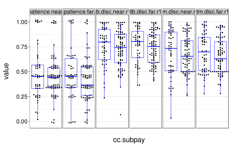
Relationships between econometric measures

We will consider only round 1.

rd(d = 2, abbcor(ss(sb, good & tv %in% 5:8)[qw(itf.patience.near.r1, itb.disc.near.r1, itm.disc.near.r1)],
    method = "kendall"))

	itb.disc.near.r1	itm.disc.near.r1
itf.patience.near.r1	0.65	0.46
itb.disc.near.r1		0.48

rd(d = 2, abbcor(ss(sb, good & tv %in% 5:8)[qw(itf.patience.far.r1, itb.disc.far.r1, itm.disc.far.r1)],
    method = "kendall"))

	itb.disc.far.r1	itm.disc.far.r1
itf.patience.far.r1	0.55	0.42
itb.disc.far.r1		0.49

It looks like the different measures are generally related to each other, but not so tightly that one can be inferred from another. Good, that's what I expected.

Convergent prediction

convergent.validity = function(dist, ses)
   {linreg.r2 = function(iv, dv, min.y, max.y)
       {pred = crossvalid(iv, dv, nfold = 10, f = function(train.iv, train.dv, test.iv)
           {model = lm(y ~ x, data.frame(x = train.iv, y = train.dv))
            predict(model, newdata = data.frame(x = test.iv))})
        pred = pmin(max.y, pmax(min.y, pred))
        1 - sum((dv - pred)^2) / sum((dv - mean(dv))^2)}
    nameify = function(f, x)
        f(x, qw(Fixed, Bisection, Matching))
    nameify(`rownames<-`, nameify(`colnames<-`, rd(d = 2, 
        do.call(cbind, lapply(list(itf.scores, itb.discs, itm.discs), function(dv.d)
           {sapply(list(itf.scores, itb.discs, itm.discs), function(iv.d)
               {if (identical(iv.d, dv.d))
                    return(NA)
                iv = ss(iv.d, s %in% ses & round == "round1" & type == dist)[,ncol(iv.d)]
                dv = ss(dv.d, s %in% ses & round == "round1" & type == dist)[,ncol(dv.d)]
                linreg.r2(iv, dv,
                    min.y = 0,
                    max.y = if (identical(dv.d, itf.scores)) 20 else 1)})})))))}

convergent.validity("near", good.s.5to8)

	Fixed	Bisection	Matching
Fixed		0.51	0.30
Bisection	0.52		0.34
Matching	0.31	0.34

convergent.validity("far", good.s.5to8)

	Fixed	Bisection	Matching
Fixed		0.41	0.24
Bisection	0.40		0.43
Matching	0.24	0.44

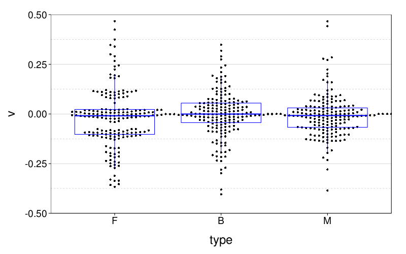
Stationarity

We will get stationarity scores, or rather, nonstationarity scores, by subtracting patience with a 30-day front-end delay from patience with no front-end delay. If far - near > 0, then far > near, so people are more patient in the far case, so positive scores on these measures mean classicial nonstationarity (being more patient in the future than the present) and negative scores mean backwards nonstationarity.

d = with(ss(dfn(sb), good & tv %in% 5:8), rbind(
    data.frame(type = "F", s = RNAME, v = itf.patience.far.r1 - itf.patience.near.r1),
    data.frame(type = "B", s = RNAME, v = itb.disc.far.r1 - itb.disc.near.r1),
    data.frame(type = "M", s = RNAME, v = itm.disc.far.r1 - itm.disc.near.r1)))

First, the count of subjects with each nonstationarity direction for each measure.

t(daply(d, .(type), function(d) table(factor(sign(d$v), levels = c(-1, 0, 1)))))

	F	B	M
-1	75	95	100
0	64	0	10
1	42	86	71

Surprisingly, backwards nonstationarity is more common than classical nonstationarity. This replicates Sayman and Öncüler's (2009) finding for (real, longitudinally observed) dynamic inconsistency.

Here is a (not terribly useful) figure.

dodge(type, v, data = transform(d, v = ifelse(type == "F",
      v/20 + runif(nrow(d), -.025, .025),
      v))) +
   coord_cartesian(ylim = c(-.5, .5)) +
   boxp

This information is more easily digested from a table of quantiles.

t(daply(d, .(type), function(d) rd(quantile(d$v, c(.025, .25, .5, .75, .975)))))

	F	B	M
2.5%	-7.000	-0.254	-0.189
25%	-2.000	-0.044	-0.067
50%	0.000	-0.001	-0.008
75%	0.000	0.055	0.031
97.5%	7.000	0.282	0.275

We see that for the most part, nonstationarity was small. That is, subjects' choices were not much affected by the front-end delay. Here are quantiles for the absolute differences:

t(daply(d, .(type), function(d) rd(quantile(abs(d$v), c(.25, .5, .75, .95)))))

	F	B	M
25%	0.000	0.017	0.015
50%	2.000	0.051	0.048
75%	3.000	0.115	0.098
95%	7.000	0.275	0.224

Concordance of stationarity between families

Here's the percent of stationarity scores that agreed in sign:

sign.agreement = function(d, t1, t2)
   `names<-`(mean(sign(ss(d, type == t1)$v) == sign(ss(d, type == t2)$v)),
       paste(t1, "and", t2))

rd(c(
   sign.agreement(d, "F", "B"),
   sign.agreement(d, "F", "M"),
   sign.agreement(d, "B", "M")))

	value
F and B	0.337
F and M	0.376
B and M	0.519

Presumably the comparisons involving F have clearly lower percentages than the comparison between B and M because only in the fixed test, due to its discrete nature, could one readily get a stationarity score of 0.

Removing all subjects from the dataset with stationarity 0 in any family yields:

d2 = ss(d, !(s %in% ss(d, v == 0)$s))
c("New sample size" = length(unique(d2$s)))

	value
New sample size	112

Now let's redo the sign-agreement analysis:

d2 = ss(d, !(s %in% ss(d, v == 0)$s))

rd(c(
   sign.agreement(d2, "F", "B"),
   sign.agreement(d2, "F", "M"),
   sign.agreement(d2, "B", "M")))

	value
F and B	0.518
F and M	0.562
B and M	0.545

Now the three figures look about the same.

Here are Kendall correlations of stationarity scores (back to including subjects with stationarity 0):

mag.corr = function(t1, t2)
   `names<-`(cor(ss(d, type == t1)$v, ss(d, type == t2)$v, method = "kendall"),
       paste(t1, "and", t2))

rd(c(
   mag.corr("F", "B"),
   mag.corr("F", "M"),
   mag.corr("B", "M")))

	value
F and B	0.059
F and M	0.032
B and M	0.064

Those look very small. At least they're all positive.

Predicting the criterion variables

A correlation matrix of the criterion variables

round(d = 2, abbcor(
    sb[good.s, qw(bmi, exercise, healthy.meals, savings,
        tobacco, gambling, floss, cc.latefees, cc.subpay)],
    method = "kendall",
    use = "complete.obs"))

	exercise	healthy.meals	savings	tobacco	gambling	floss	cc.latefees	cc.subpay
bmi	-0.07	-0.08	-0.09	0.03	0.09	-0.02	0.05	0.10
exercise		0.23	-0.03	0.11	0.03	0.13	0.09	-0.01
healthy.meals			0.15	-0.03	-0.08	0.16	-0.06	0.04
savings				-0.01	0.06	0.11	-0.17	-0.22
tobacco					0.15	0.05	-0.06	-0.04
gambling						-0.03	0.00	-0.02
floss							-0.04	-0.10
cc.latefees								0.31

Possibly one could use this correlation matrix to make loose inferences about the maximum predictability of the criterion variables using some other variable, the logic being that if there is some other variable that can predict all of them, they necessarily should be predictable from each other. But it's complicated.

Preparing the criterion variables

BMI is negatively skewed:

dodge(1, ss(sb, good & tv %in% 5:8)$bmi)

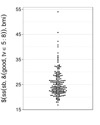
So let's use the logarithm instead, and also clip that high point down to the second-highest point. I wouldn't consider it an outlier, but I don't want to overweight an extreme value like that, for training or for testing.

For smoking, the number of packs of cigarettes has a funny-looking distribution:

table(ss(sb, good & tv %in% 5:8)$cigpacks, useNA = "always")

	count
0	1
1	3
2	10
3	8
4	5
5	2
6	2
7	11
14	2
NA	137

Let's stick to predicting just whether or not the subject uses tobacco, at least to begin with.

For gambling and late fees for paying off credit cards, let us also do dichtomous prediction, since so few of our subjects endorse a count above 0 for either:

table(ss(sb, good & tv %in% 5:8)$gambling > 0)

	count
FALSE	150
TRUE	31

table(ss(sb, good & tv %in% 5:8)$cc.latefees > 0, useNA = "always")

	count
FALSE	100
TRUE	34
NA	47

Notice that, surprisingly, more subjects lack a credit card entirely than admit to having paid even one late fee in the past two years.

Exercise, like BMI, is negatively skewed:

dodge(1, exercise, data = ss(sb, good & tv %in% 5:8))

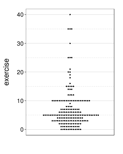
So we'll again use the logarithm (plus one to compensate for zeroes).

For healthy eating, as well as for a few other variables, subjects could enter one of 0%, 1%, 2%, …, 100%. This prohibits immediate use of a logistic transformation (since $\operatorname{logit} 0$ and $\operatorname{logit} 1$ are infinite). We will clip 0% to 0.5% and 100% to 99.5% before applying $\operatorname{logit}$ .

Flossing has another odd distribution, which suggests a tripartite representation:

with(ss(sb, good & tv %in% 5:8), table(ordered(
    ifelse(floss == 0, "<weekly", 
        ifelse(floss < 7, "<daily", ">=daily")),
    levels = c("<weekly", "<daily", ">=daily"))))

	count
<weekly	53
<daily	63
>=daily	65

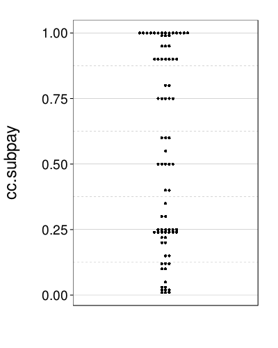
For cc.subpay, most subjects with credit cards admit to sub-paying at least once in the last two years…

with(ss(sb, good & tv %in% 5:8), table(cc.subpay > 0))

	count
FALSE	53
TRUE	81

…but the distribution for cc.subpay > 0 is odd, so I think I'll stick to dichotomous prediction.

dodge(1, cc.subpay, data = ss(sb, good & tv %in% 5:8 &
    !is.na(cc.subpay) & cc.subpay > 0))

We'll treat savings like healthy.meals except that we'll clip a single very high point, as for BMI.

sb2 = within(ss(sb, good & tv %in% 5:8),
   {bmi[which.max(bmi)] = sort(bmi, dec = T)[2]
    bmi = log(bmi)
    gambling = gambling > 0
    exercise = log(exercise + 1)
    healthy.meals = logit(pmin(.995, pmax(.005, healthy.meals)))
    floss = ordered(
        ifelse(floss == 0, "<weekly", 
            ifelse(floss < 7, "<daily", ">=daily")),
        levels = c("<weekly", "<daily", ">=daily"))
    cc.latefees = cc.latefees > 0
    cc.subpay = cc.subpay > 0
    savings[which.max(savings)] = sort(savings, dec = T)[2]
    savings = logit(pmin(.995, pmax(.005, savings)))})

vlist = list(
    c("bmi", "ols"),
    c("exercise", "ols"),
    c("healthy.meals", "ols"),
    c("savings", "ols"),
    c("tobacco", "logistic"),
    c("gambling", "logistic"),
    c("floss", "ordinal"),
    # Perform the credit card-related analyses on just the subjects
    # who said they have a credit card.
    c("cc.latefees", "logistic", "remove.nas"),
    c("cc.subpay", "logistic", "remove.nas"))

discrete.vlist = Filter(function(x) x[[2]] == "logistic" || x[[2]] == "ordinal", vlist)
continuous.vlist = Filter(function(x) x[[2]] == "ols", vlist)

First try

m = sapply(vlist, function(x)
   {var = x[1]
    modeltype = x[2]
    remove.nas = length(x) >= 3
    sbf = if (remove.nas) sb2[!is.na(sb2[[var]]),] else sb2
    y = sbf[[var]]
    rd(c((if (modeltype == "logistic") max(mean(y), 1 - mean(y))
        else if (modeltype == "ordinal") max(prop.table(tabulate(y)))
        else sd(y)),
        sapply(qw(itf.patience, itb.disc, itm.disc), function(s)
       {d = sbf[paste0(s, c(".near.r1", ".far.r1"))]
        names(d) = qw(near, far)
        if (modeltype == "logistic")
           {pred = crossvalid(d, y, nfold = 10, f = function(train.iv, train.dv, test.iv)
               {model = glm(y ~ near * far, cbind(train.iv, y = train.dv),
                    family = binomial(link = "logit"))
                predict(model, type = "response", newdata = test.iv)})
            mean((pred >= .5) == y)}
        else if (modeltype == "ordinal")
           {pred = crossvalid(d, y, nfold = 10, f = function(train.iv, train.dv, test.iv)
               {model = polr(y ~ near * far, cbind(train.iv, y = train.dv),
                    method = "logistic")
                char(predict(model, type = "class", newdata = test.iv))})
            mean(pred == char(y))}
        else
           {pred = crossvalid(d, y, nfold = 10, f = function(train.iv, train.dv, test.iv)
               {model = lm(y ~ near * far, cbind(train.iv, y = train.dv))
                predict(model, newdata = test.iv)})
            sqrt(mean( (pred - y)^2 ))}})))})

colnames(m) = sapply(vlist, function(x) x[[1]])
m

	bmi	exercise	healthy.meals	savings	tobacco	gambling	floss	cc.latefees	cc.subpay
	0.181	0.793	2.701	1.840	0.757	0.829	0.359	0.746	0.604
itf.patience	0.186	0.803	2.704	1.877	0.757	0.823	0.304	0.731	0.582
itb.disc	0.185	0.767	2.739	1.845	0.757	0.829	0.370	0.731	0.604
itm.disc	0.186	0.806	2.721	1.864	0.757	0.823	0.331	0.739	0.575

In this table, the top row measures base variability (the SD for continuous variables, and the base rate of the modal class for discrete variables), and the other rows indicate cross-validation estimates of test error (the RMSE for continuous variables, and the correct classification rate for discrete variables).

Surprisingly, despite good preliminary evidence that our econometric tests are reliable (in terms of immediate test–retest reliability and intercorrelations between tests), none of these simple analyses with the criterion variables as DV came close to working. In fact, the only improvement I see in the above table is that the itb-based model predicting exercise achieved a RMSE of .77 compared to the SD of .79. This is not a meaningful improvement. Either the econometric tests are quite useless for predicting the criterion variables, or we need fancier models. Let's try fancier models.

Discrete criterion variables

First, plots. These are crude but hopefully better than nothing.

its = qw(itf.patience.near.r1, itf.patience.far.r1,
    itb.disc.near.r1, itb.disc.far.r1,
    itm.disc.near.r1, itm.disc.far.r1)
dichot.plot.df = transform(
    melt(sb2[c(its, qw(tobacco, gambling, cc.latefees, cc.subpay))],
        id.vars = qw(tobacco, gambling, cc.latefees, cc.subpay)),
    value = ifelse(
        variable %in% qw(itf.patience.near.r1, itf.patience.far.r1),
        value/20 + runif(length(value), -.02, .02),
        value))
dichot.plot = function(var, drop.nas = F)
  {if (drop.nas)
       dichot.plot.df = dichot.plot.df[!is.na(dichot.plot.df[[char(var)]]),]
   eval(bquote(dodge(.(var), value, faceter = variable, data = dichot.plot.df))) +
       scale_x_discrete(breaks = c(0, 1)) +
       coord_cartesian(xlim = c(.5, 2.5)) +
       boxp}

dichot.plot(quote(tobacco))

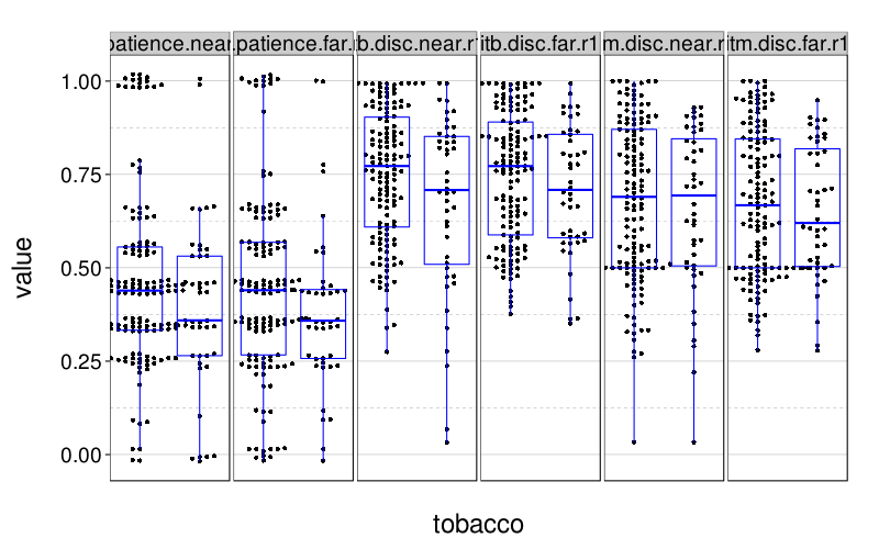
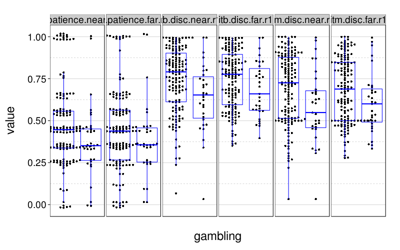
dichot.plot(quote(gambling))

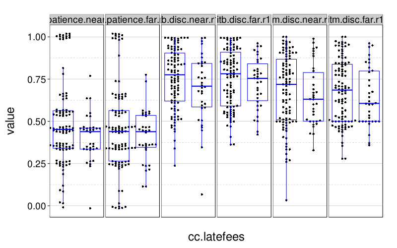
dichot.plot(quote(cc.latefees), drop.nas = T)

dichot.plot(quote(cc.subpay), drop.nas = T)

These look a little better than the first-try analyses above suggested.

Let's try nearest-neighbors:

m = rd(sapply(discrete.vlist, function(x)
   {var = x[1]
    remove.nas = length(x) >= 3
    sbf = if (remove.nas) sb2[!is.na(sb2[[var]]),] else sb2
    y = sbf[[var]]
    if (is.ordered(y))
        class(y) = "factor"
    c(max(prop.table(table(y))), sapply(qw(itf.patience, itb.disc, itm.disc), function(s)
       {near = sbf[[paste0(s, ".near.r1")]]
        far = sbf[[paste0(s, ".far.r1")]]
        # Since 'near' and 'far' are two slight variations of the
        # same test, we won't rescale them.
        pred = crossvalid(cbind(near, far), y, nfold = 10,
            f = function(train.iv, train.dv, test.iv)
               knn.autok(train.iv, test.iv, train.dv))
        mean(pred == y)}))}))

colnames(m) = sapply(discrete.vlist, function(x) x[[1]])
m

	tobacco	gambling	floss	cc.latefees	cc.subpay
	0.757	0.829	0.359	0.746	0.604
itf.patience	0.740	0.812	0.271	0.709	0.552
itb.disc	0.768	0.790	0.238	0.709	0.507
itm.disc	0.707	0.790	0.343	0.694	0.515

The cross-validatory estimates of test-set accuracy are, with one small exception, lower than the base rate of the modal class. So much for that.

How about random forests?

m = rd(sapply(discrete.vlist, function(x)
   {var = x[1]
    remove.nas = length(x) >= 3
    sbf = if (remove.nas) sb2[!is.na(sb2[[var]]),] else sb2
    y = factor(sbf[[var]])
    if (is.ordered(y))
        class(y) = "factor"
    c(max(prop.table(table(y))), sapply(qw(itf.patience, itb.disc, itm.disc), function(s)
       {near = sbf[[paste0(s, ".near.r1")]]
        far = sbf[[paste0(s, ".far.r1")]]
        rf = randomForest(x = cbind(near, far), y = y,
            ntree = 2000,
            mtry = 2) # Since there are only two predictors.
        1 - tail(rf$err.rate, 1)[1]}))}))

colnames(m) = sapply(discrete.vlist, function(x) x[[1]])
m

	tobacco	gambling	floss	cc.latefees	cc.subpay
	0.757	0.829	0.359	0.746	0.604
itf.patience	0.713	0.785	0.376	0.642	0.545
itb.disc	0.773	0.757	0.298	0.672	0.470
itm.disc	0.685	0.724	0.414	0.657	0.500

This time we have only two cases for which estimated test-set accuracy exceeds the base rate of the modal class. One of these, itm used to predict flossing, is large enough to be meaningful (41% versus 36%) but still quite small.

How about SVMs?

m = rd(sapply(discrete.vlist, function(x)
   {var = x[1]
    remove.nas = length(x) >= 3
    sbf = if (remove.nas) sb2[!is.na(sb2[[var]]),] else sb2
    y = sbf[[var]]
    if (is.ordered(y))
        class(y) = "factor"
    c(max(prop.table(table(y))), sapply(qw(itf.patience, itb.disc, itm.disc), function(s)
       {near = sbf[[paste0(s, ".near.r1")]]
        far = sbf[[paste0(s, ".far.r1")]]
        # Since 'near' and 'far' are two slight variations of the
        # same test, we won't rescale them.
        pred = crossvalid(cbind(near, far), y, nfold = 10,
            f = function(train.iv, train.dv, test.iv)
               {model = best.svm(x = train.iv, y = train.dv,
                    scale = F, type = "C-classification",
                    gamma = 10^(-6:-6),
                    cost = 10^(-6:6))
                char(predict(model, test.iv))})
        mean(pred == char(y))}))}))

colnames(m) = sapply(discrete.vlist, function(x) x[[1]])
m

	tobacco	gambling	floss	cc.latefees	cc.subpay
	0.757	0.829	0.359	0.746	0.604
itf.patience	0.757	0.829	0.271	0.746	0.604
itb.disc	0.757	0.829	0.287	0.746	0.604
itm.disc	0.757	0.829	0.265	0.746	0.604

At their best, the SVMs are constantly predicting the modal class.

Using a scoring rule

mean.nll2 = function(pv, outcomes)
    mean(-log( ifelse(outcomes, pv, 1 - pv), 2 ))

f = function(vname, modeltype, na.rm = F)
   {sbf = if (na.rm) sb2[!is.na(sb2[[vname]]),] else sb2
    y = sbf[[vname]]
    if (is.logical(y))
        y = num(y)
    round(digits = 2, c(mean.nll2(mean(y), y),
        sapply(qw(itf.patience, itb.disc, itm.disc), function(s)
       {d = sbf[paste0(s, c(".near.r1", ".far.r1"))]
        names(d) = qw(near, far)
        if (modeltype == "binary")
           {pred = crossvalid(d, y, nfold = 10, f = function(train.iv, train.dv, test.iv)
               {model = glm(y ~ near * far, cbind(train.iv, y = train.dv),
                    family = binomial(link = "logit"))
                predict(model, type = "response", newdata = test.iv)})
            mean.nll2(pred, y)}})))}
m = data.frame(check.names = F,
    "Tobacco use" = f("tobacco", "binary"),
    Gambling = f("gambling", "binary"),
    "CC late fees" = f("cc.latefees", "binary", na.rm = T),
    "CC subpayment" = f("cc.subpay", "binary", na.rm = T))
m = rbind(m[1,], NA, m[-1,])
m

	Tobacco use	Gambling	CC late fees	CC subpayment
	0.80	0.66	0.82	0.97
2
itf.patience	0.81	0.68	0.82	0.99
itb.disc	0.81	0.65	0.84	1.02
itm.disc	0.82	0.68	0.89	0.98

No improvement.

Continuous criterion variables

Kernel regression:

m = rd(sapply(continuous.vlist, function(x)
   {var = x[1]
    remove.nas = length(x) >= 3
    sbf = if (remove.nas) sb2[!is.na(sb2[[var]]),] else sb2
    y = sbf[[var]]
    c(sd(y), sapply(qw(itf.patience, itb.disc, itm.disc), function(s)
       {iv = sbf[paste0(s, qw(.near.r1, .far.r1))]
        names(iv) = qw(near, far)
        pred = crossvalid(iv, y, nfold = 10,
            f = function(train.iv, train.dv, test.iv)
              {d = data.frame(train.iv, y = train.dv)
               predict(
                   npreg(y ~ near + far, data = d,
                       regtype = "ll", ckertype = "epanechnikov"),
                   newdata = test.iv)})
        sqrt(mean((pred - y)^2))}))}))

colnames(m) = sapply(continuous.vlist, function(x) x[[1]])
m

	bmi	exercise	healthy.meals	savings
	0.181	0.793	2.701	1.840
itf.patience	0.184	0.820	2.733	1.939
itb.disc	0.183	0.772	2.712	1.853
itm.disc	0.190	0.832	2.661	1.938

It looks like this kernel-regression technique did even worse than linear regression.

Let's try random forests again:

m = rd(sapply(continuous.vlist, function(x)
   {var = x[1]
    remove.nas = length(x) >= 3
    sbf = if (remove.nas) sb2[!is.na(sb2[[var]]),] else sb2
    y = sbf[[var]]
    c(sd(y), sapply(qw(itf.patience, itb.disc, itm.disc), function(s)
       {near = sbf[[paste0(s, ".near.r1")]]
        far = sbf[[paste0(s, ".far.r1")]]
        rf = randomForest(x = cbind(near, far), y = y,
            ntree = 2000,
            mtry = 2) # Since there are only two predictors.
        sqrt(mean((rf$predicted - y)^2))}))}))

colnames(m) = sapply(continuous.vlist, function(x) x[[1]])
m

	bmi	exercise	healthy.meals	savings
	0.181	0.793	2.701	1.840
itf.patience	0.201	0.882	3.058	2.028
itb.disc	0.208	0.815	2.965	2.040
itm.disc	0.206	0.804	2.874	2.109

Shoot, that was really bad.

Association and significance testing

Correlation tests and t-tests

For the continuous criterion variables (and also flossing), we do Pearson correlation tests.

m = do.call(rbind, lapply(c(continuous.vlist, list("floss")), function(x)
   {dv = x[1]
    y = num(sb2[[dv]])
    cbind(dv, do.call(rbind, lapply(qw(itf.patience.near.r1, itf.patience.far.r1, itb.disc.near.r1, itb.disc.far.r1, itm.disc.near.r1, itm.disc.far.r1), function(iv)
       {ct = cor.test(sb2[,iv], y, method = "pearson")
        data.frame(iv,
            r = round(ct$estimate, 2),
            p = round(ct$p.value, 3),
            s = (if (ct$p.value < .05) "*" else ""))})))}))
rownames(m) = c()
m

	dv	iv	r	p	s
1	bmi	itf.patience.near.r1	-0.01	0.885
2	bmi	itf.patience.far.r1	0.04	0.567
3	bmi	itb.disc.near.r1	0.03	0.686
4	bmi	itb.disc.far.r1	-0.02	0.778
5	bmi	itm.disc.near.r1	-0.02	0.740
6	bmi	itm.disc.far.r1	-0.01	0.887
7	exercise	itf.patience.near.r1	-0.10	0.191
8	exercise	itf.patience.far.r1	-0.11	0.126
9	exercise	itb.disc.near.r1	-0.25	0.001	*
10	exercise	itb.disc.far.r1	-0.10	0.199
11	exercise	itm.disc.near.r1	-0.16	0.030	*
12	exercise	itm.disc.far.r1	-0.19	0.012	*
13	healthy.meals	itf.patience.near.r1	0.00	0.974
14	healthy.meals	itf.patience.far.r1	-0.03	0.690
15	healthy.meals	itb.disc.near.r1	0.00	0.990
16	healthy.meals	itb.disc.far.r1	0.11	0.127
17	healthy.meals	itm.disc.near.r1	0.13	0.077
18	healthy.meals	itm.disc.far.r1	0.12	0.112
19	savings	itf.patience.near.r1	0.04	0.567
20	savings	itf.patience.far.r1	0.06	0.432
21	savings	itb.disc.near.r1	0.09	0.216
22	savings	itb.disc.far.r1	0.16	0.037	*
23	savings	itm.disc.near.r1	0.10	0.171
24	savings	itm.disc.far.r1	0.07	0.321
25	floss	itf.patience.near.r1	0.08	0.313
26	floss	itf.patience.far.r1	0.07	0.377
27	floss	itb.disc.near.r1	0.07	0.319
28	floss	itb.disc.far.r1	0.06	0.412
29	floss	itm.disc.near.r1	0.09	0.251
30	floss	itm.disc.far.r1	0.11	0.159

For the dichotomous criterion variables, we do t-tests, treating the criterion variables as independent (grouping) variables and time preferences as dependent variables.

m = do.call(rbind, lapply(discrete.vlist, function(x)
   {dv = x[1]
    modeltype = x[2]
    if (modeltype == "ordinal")
        return(data.frame())
    na.rm = length(x) >= 3
    sbf = if (na.rm) sb2[!is.na(sb2[[dv]]),] else sb2
    y = num(sbf[[dv]])
    cbind(iv = dv, do.call(rbind, lapply(qw(itf.patience.near.r1, itf.patience.far.r1, itb.disc.near.r1, itb.disc.far.r1, itm.disc.near.r1, itm.disc.far.r1), function(iv)
       {tt = t.test(var.eq = T, sb2[y == 0, iv], sb2[y == 1, iv])
        data.frame(dv = iv,
            p = round(tt$p.value, 3),
            s = (if (tt$p.value < .05) "*" else ""))})))}))
rownames(m) = c()
m

	iv	dv	p	s
1	tobacco	itf.patience.near.r1	0.079
2	tobacco	itf.patience.far.r1	0.177
3	tobacco	itb.disc.near.r1	0.023	*
4	tobacco	itb.disc.far.r1	0.207
5	tobacco	itm.disc.near.r1	0.526
6	tobacco	itm.disc.far.r1	0.503
7	gambling	itf.patience.near.r1	0.065
8	gambling	itf.patience.far.r1	0.177
9	gambling	itb.disc.near.r1	0.004	*
10	gambling	itb.disc.far.r1	0.069
11	gambling	itm.disc.near.r1	0.007	*
12	gambling	itm.disc.far.r1	0.054
13	cc.latefees	itf.patience.near.r1	0.445
14	cc.latefees	itf.patience.far.r1	0.550
15	cc.latefees	itb.disc.near.r1	0.470
16	cc.latefees	itb.disc.far.r1	0.981
17	cc.latefees	itm.disc.near.r1	0.324
18	cc.latefees	itm.disc.far.r1	0.208
19	cc.subpay	itf.patience.near.r1	0.620
20	cc.subpay	itf.patience.far.r1	0.083
21	cc.subpay	itb.disc.near.r1	0.352
22	cc.subpay	itb.disc.far.r1	0.124
23	cc.subpay	itm.disc.near.r1	0.162
24	cc.subpay	itm.disc.far.r1	0.059

Regression

Now we do significance tests with the models we used for the predictive analyses.

m = do.call(rbind, lapply(c(continuous.vlist, list("floss")), function(x)
   {dv = x[1]
    y = num(sb2[[dv]])
    cbind(dv, do.call(rbind, lapply(qw(itf.patience, itb.disc, itm.disc), function(s)
       {d = data.frame(
           near = scale(sb2[[paste0(s, ".near.r1")]]),
           far = scale(sb2[[paste0(s, ".far.r1")]]))
        cm = coef(summary(lm(y ~ near * far, data = d)))[-1,]
#        cat(dv, s, round(d = 3, summary(lm(y ~ near * far, data = d))$r.squared), "\n")
        data.frame(
            ivs = (if (s == "itf.patience") "fixed"
               else if (s == "itb.disc") "bisection"
               else "matching"),
            coef = rownames(cm),
            p = round(d = 3, cm[,"Pr(>|t|)"]),
            s = ifelse(cm[,"Pr(>|t|)"] < .05, "*", ""))})))}))
rownames(m) = c()
m

	dv	ivs	coef	p	s
1	bmi	fixed	near	0.447
2	bmi	fixed	far	0.292
3	bmi	fixed	near:far	0.861
4	bmi	bisection	near	0.379
5	bmi	bisection	far	0.408
6	bmi	bisection	near:far	0.956
7	bmi	matching	near	0.687
8	bmi	matching	far	0.784
9	bmi	matching	near:far	0.972
10	exercise	fixed	near	0.443
11	exercise	fixed	far	0.357
12	exercise	fixed	near:far	0.131
13	exercise	bisection	near	0.000	*
14	exercise	bisection	far	0.102
15	exercise	bisection	near:far	0.241
16	exercise	matching	near	0.997
17	exercise	matching	far	0.201
18	exercise	matching	near:far	0.893
19	healthy.meals	fixed	near	0.188
20	healthy.meals	fixed	far	0.672
21	healthy.meals	fixed	near:far	0.012	*
22	healthy.meals	bisection	near	0.067
23	healthy.meals	bisection	far	0.031	*
24	healthy.meals	bisection	near:far	0.029	*
25	healthy.meals	matching	near	0.712
26	healthy.meals	matching	far	0.546
27	healthy.meals	matching	near:far	0.045	*
28	savings	fixed	near	0.939
29	savings	fixed	far	0.580
30	savings	fixed	near:far	0.766
31	savings	bisection	near	0.681
32	savings	bisection	far	0.089
33	savings	bisection	near:far	0.796
34	savings	matching	near	0.397
35	savings	matching	far	0.851
36	savings	matching	near:far	0.530
37	floss	fixed	near	0.396
38	floss	fixed	far	0.806
39	floss	fixed	near:far	0.316
40	floss	bisection	near	0.571
41	floss	bisection	far	0.892
42	floss	bisection	near:far	0.889
43	floss	matching	near	0.867
44	floss	matching	far	0.386
45	floss	matching	near:far	0.756

m = do.call(rbind, lapply(c(discrete.vlist), function(x)
   {dv = x[1]
    modeltype = x[2]
    if (modeltype == "ordinal")
        return(data.frame())
    na.rm = length(x) >= 3
    sbf = if (na.rm) sb2[!is.na(sb2[[dv]]),] else sb2
    y = num(sbf[[dv]])
    cbind(dv, do.call(rbind, lapply(qw(itf.patience, itb.disc, itm.disc), function(s)
       {d = data.frame(
           near = scale(sbf[[paste0(s, ".near.r1")]]),
           far = scale(sbf[[paste0(s, ".far.r1")]]))
        cm = coef(summary(glm(y ~ near * far, data = d, family = binomial)))[-1,]
        predps = predict(
            glm(y ~ near * far, data = d, family = binomial(link = "probit")),
            type = "response")
        cat(dv, s, round(d = 3, 1 -
            sum((y - predps)^2) / sum((y - mean(y))^2)), "\n")
        data.frame(
            ivs = (if (s == "itf.patience") "fixed"
               else if (s == "itb.disc") "bisection"
               else "matching"),
            coef = rownames(cm),
            p = round(d = 3, cm[,"Pr(>|z|)"]),
            s = ifelse(cm[,"Pr(>|z|)"] < .05, "*", ""))})))}))
rownames(m) = c()
m

	dv	ivs	coef	p	s
1	tobacco	fixed	near	0.211
2	tobacco	fixed	far	0.934
3	tobacco	fixed	near:far	0.680
4	tobacco	bisection	near	0.063
5	tobacco	bisection	far	0.607
6	tobacco	bisection	near:far	0.699
7	tobacco	matching	near	0.856
8	tobacco	matching	far	0.852
9	tobacco	matching	near:far	0.763
10	gambling	fixed	near	0.112
11	gambling	fixed	far	0.986
12	gambling	fixed	near:far	0.264
13	gambling	bisection	near	0.029	*
14	gambling	bisection	far	0.802
15	gambling	bisection	near:far	0.201
16	gambling	matching	near	0.065
17	gambling	matching	far	0.662
18	gambling	matching	near:far	0.908
19	cc.latefees	fixed	near	0.346
20	cc.latefees	fixed	far	0.751
21	cc.latefees	fixed	near:far	0.186
22	cc.latefees	bisection	near	0.137
23	cc.latefees	bisection	far	0.767
24	cc.latefees	bisection	near:far	0.220
25	cc.latefees	matching	near	0.967
26	cc.latefees	matching	far	0.680
27	cc.latefees	matching	near:far	0.269
28	cc.subpay	fixed	near	0.727
29	cc.subpay	fixed	far	0.294
30	cc.subpay	fixed	near:far	0.931
31	cc.subpay	bisection	near	0.649
32	cc.subpay	bisection	far	0.674
33	cc.subpay	bisection	near:far	0.474
34	cc.subpay	matching	near	0.347
35	cc.subpay	matching	far	0.200
36	cc.subpay	matching	near:far	0.129

Session 2

Planning

If 30 days is a good retest interval, since that's the front-end delay, let's try to start rerunning subjects 30 days, on average, since we first ran them.

I'm thinking of doing 5 waves of admitting 10 subjects per day (at 9 am, noon, 3 pm, 6 pm, and 9 pm). Everyone will then be admitted over the course of four days.

do.call(c, lapply(list(1:50, 51:100, 101:150, 151:200), function(i)
    median(as.Date(ss(sb, tv %in% 5:8)$began_t)[i] + 30)))

	x
1	2014-03-18
2	2014-03-20
3	2014-03-21
4	2014-03-22

Let's admit everyone on weekdays to reduce the chance of a weekend rush. That makes the appropriate days Tuesday, March 18 through Friday, March 21. We can make the HIT end on Monday evening (the 24th).

For implementation, let's use a fresh database and match up subject numbers (using worker IDs) post hoc. Let us also try to make the keys in the User table not overlap with any of those from last time so the User tables from the two databases can be easily merged once subject numbers have been corrected.

The HIT will require a Qualification that we'll grant to workers at the same time we notify them that the new HIT exists.

Score-for-score reliability

How well can we predict scores in rounds 2 and 3 using exactly the scores from round 1, with no model or other fanciness?

score.for.score.pred = function(dv, ses)
    `colnames<-`(value = qw(F.near, F.far, B.near, B.far, M.near, M.far), round(d = 2,
        do.call(cbind, lapply(list(itf.scores, itb.discs, itm.discs), function(d)
            t(aaply(acast(ss(d, s %in% ses), s ~ type ~ round), c(2), function(a) c(
#                SD = sd(a[,dv]),
#                RMSE = sqrt(mean((a[,dv] - a[,"round1"])^2)),
                PVAF = 1 - sum((a[,dv] - a[,"round1"])^2)/sum((a[,dv] - mean(a[,dv]))^2),
                "Abs err, median" = median(abs(a[,dv] - a[,"round1"])),
                "Abs err, .9 q" = num(quantile(abs(a[,dv] - a[,"round1"]), .9)),
                "Abs err, .95 q" = num(quantile(abs(a[,dv] - a[,"round1"]), .95)),
                Bias = mean(a[,"round1"] - a[,dv]),
                Kendall = cor(a[,dv], a[,"round1"], method = "kendall"),
                Pearson = cor(a[,dv], a[,"round1"]))))))))

score.for.score.pred("round2", good.s)

	F.near	F.far	B.near	B.far	M.near	M.far
PVAF	0.70	0.49	0.53	0.64	0.78	0.82
Abs err, median	2.00	2.00	0.04	0.05	0.03	0.03
Abs err, .9 q	5.00	7.00	0.23	0.18	0.14	0.14
Abs err, .95 q	5.00	9.00	0.28	0.24	0.19	0.18
Bias	0.10	0.09	0.00	-0.01	-0.01	-0.01
Kendall	0.71	0.61	0.65	0.64	0.75	0.77
Pearson	0.85	0.72	0.77	0.81	0.89	0.91

score.for.score.pred("round3", good.s.s2)

	F.near	F.far	B.near	B.far	M.near	M.far
PVAF	0.44	0.57	0.44	0.64	0.57	0.56
Abs err, median	2.00	2.00	0.06	0.04	0.06	0.05
Abs err, .9 q	5.00	5.00	0.16	0.19	0.19	0.21
Abs err, .95 q	7.00	6.00	0.21	0.23	0.28	0.26
Bias	-0.37	-0.29	0.01	0.01	-0.02	-0.02
Kendall	0.66	0.65	0.66	0.67	0.65	0.62
Pearson	0.77	0.80	0.72	0.82	0.81	0.79

Judging from the PVAFs and considering that matching is the quickest and easiest test, perhaps matching is best. Matching also has the advantage that it is intuitive how lengthening the test should improve reliability.

Let's use a similar strategy to investigate nonstationarity by examining how well round-1 near scores predict round-2 far scores. (We use the DV from round 2 rather than 1 for better comparability with the first analysis.)

`colnames<-`(value = qw(F, B, M), round(d = 2,
    do.call(cbind, lapply(list(itf.scores, itb.discs, itm.discs), function(d)
       {iv = ss(d, s %in% good.s.s2 & round == "round1" & type == "near")[,ncol(d)]
        dv = ss(d, s %in% good.s.s2 & round == "round2" & type == "far")[,ncol(d)]
        c(
#            SD = sd(dv),
#            RMSE = sqrt(mean((dv - iv)^2)),
            PVAF = 1 - sum((dv - iv)^2)/sum((dv - mean(dv))^2),
            "Abs err, median" = median(abs(dv - iv)),
            "Abs err, .9 q" = num(quantile(abs(dv - iv), .9)),
            "Abs err, .95 q" = num(quantile(abs(dv - iv), .95)),
            Bias = mean(iv - dv),
            Kendall = cor(dv, iv, method = "kendall"))}))))

	F	B	M
PVAF	0.49	0.54	0.70
Abs err, median	2.00	0.04	0.04
Abs err, .9 q	5.00	0.22	0.15
Abs err, .95 q	7.80	0.27	0.21
Bias	0.35	-0.01	0.00
Kendall	0.66	0.66	0.76

It looks like near predicts far about as well as far does. That is, the predictive validity of near for far is about as good as the reliability of far. This seems to imply it is unnecessary to measure both. You might as well measure one of them twice.

The lack of bias here is also noteworthy.

Implications for prediction

How can we estimate what these reliabilities imply for prediction?

PVAFs around .6 imply a prediction-interval reduction factor of $1 - \sqrt{1 - .6^2}$ , about 1/3. I would judge that as reasonably but not very useful for prediction. — No, wait, this calculation is fishy. The general notion of PVAF isn't the same thing as squared correlation.

By Equation (3.13) of de Gruijter and van der Kamp (2008) (p. 23), classical test theory implies that $ρ \sqrt{r} = v$ , where ρ is the correlation between true scores of the predictor and criterion, r is the reliability coefficient of the predictor, v is predictive validity, and we are assuming the criterion is perfectly reliable. So a reliability of .8 multiplies the predictor–criterion correlation by $\sqrt{.8} = .90$ . Not bad.

However, correlations are hard to interpret, so let's think about prediction-interval reduction factors (PIRFs) instead. Some algebra (in Maxima)

expr: ev((1 - sqrt(1 - v^2)), v = rho * sqrt(r))$
eq: solve(((ulpirf = 1 - sqrt(1 - rho^2)) - 1)^2, rho^2)[1]$
ev(expr, eq);

yields the formula 1-sqrt(1-r*(2*ulpirf-ulpirf^2)) to express the predictor–criterion PIRF in terms of the underyling PIRF ulpirf and the reliability coefficient r.

pirf = function(r, ulpirf) 1-sqrt(1-r*(2*ulpirf-ulpirf^2))
round(d = 2, as.matrix(transform(
    data.frame(ulpirf = c(.15, 1/4, 1/2, 3/4, .9, .99)),
    "r.6" = pirf(.6, ulpirf),
    "r.8" = pirf(.8, ulpirf))))

	ulpirf	r.6	r.8
1	0.15	0.09	0.12
2	0.25	0.14	0.19
3	0.50	0.26	0.37
4	0.75	0.34	0.50
5	0.90	0.36	0.54
6	0.99	0.37	0.55

We see that although rs of .6 and .8 severely limit the PIRF, they are enough to let the PIRF reach 1/4 and 1/3, respectively, provided ulpirf is at least 1/2. So we seem to have enough reliability to do meaningful prediction when the underlying relationship is strong, but probably not when it's moderate and certainly not when it's weak.

But see http://arfer.net/w/reliab-predacc.

Session-1 reliabilities as affected by attrition

For reviewer 2 of PaID submission 1.

Full sample:

score.for.score.pred.paper("round2", good.s.5to8)

	Near	Far	Near	Far	Near	Far
PVAF	0.70	0.49	0.51	0.62	0.75	0.82
Abs err, median	2.00	2.00	0.04	0.05	0.03	0.03
Abs err, 10th %ile	5.00	7.00	0.23	0.18	0.14	0.13
Abs err, 5th %ile	5.00	9.00	0.28	0.24	0.20	0.18
Bias	0.10	0.09	0.00	-0.01	-0.01	-0.01
Kendall τ	0.71	0.61	0.65	0.63	0.74	0.78
Pearson `r`	0.85	0.72	0.76	0.81	0.88	0.91

Returners only:

score.for.score.pred.paper("round2",
   row.names(ss(sb, good & tv %in% 5:8 & !is.na(duration.s2))))

	Near	Far	Near	Far	Near	Far
PVAF	0.72	0.67	0.63	0.71	0.82	0.89
Abs err, median	2.00	2.00	0.04	0.04	0.03	0.03
Abs err, 10th %ile	4.83	4.83	0.22	0.16	0.12	0.10
Abs err, 5th %ile	5.00	7.50	0.27	0.21	0.18	0.15
Bias	0.07	-0.19	0.01	0.00	0.00	-0.01
Kendall τ	0.74	0.73	0.67	0.68	0.77	0.82
Pearson `r`	0.86	0.82	0.81	0.85	0.91	0.95

Non-returners only:

score.for.score.pred.paper("round2",
   row.names(ss(sb, good & tv %in% 5:8 & is.na(duration.s2))))

	Near	Far	Near	Far	Near	Far
PVAF	0.63	0.23	0.33	0.49	0.63	0.71
Abs err, median	2.00	2.00	0.06	0.06	0.03	0.03
Abs err, 10th %ile	4.87	7.00	0.23	0.21	0.15	0.17
Abs err, 5th %ile	5.00	8.60	0.27	0.25	0.20	0.21
Bias	0.13	0.40	0.00	-0.02	-0.02	-0.02
Kendall τ	0.65	0.46	0.59	0.54	0.68	0.70
Pearson `r`	0.80	0.56	0.67	0.74	0.85	0.86

To my surprise, there's a clear difference: reliability was somewhat higher among the returners than the non-returners.

What does this mean for the validity results? Well, it means the comparison we invoke between the one-month retest reliabilities and predictive validities is a bit unfair, because the samples are different (particularly, the sample for which we have reliabilities is likely more reliable than the whole sample would be). So, let's examine the predictive validity among this more reliable subsample.

Continuous, original:

prederror.continuous(sb2)

	BMI	Exercise	Healthy meals	Savings
Standard deviation	5.00	6.88	0.335	0.170
Prediction error
Fixed	5.07	7.17	0.350	0.188
Bisection	5.10	6.79	0.349	0.186
Matching	5.12	7.20	0.355	0.187

Continuous, returners only:

prederror.continuous(ss(sb2, !is.na(duration.s2)))

	BMI	Exercise	Healthy meals	Savings
Standard deviation	4.93	6.80	0.333	0.163
Prediction error
Fixed	5.09	7.17	0.350	0.181
Bisection	5.11	7.01	0.352	0.179
Matching	5.15	7.38	0.377	0.181

Discrete, original:

prederror.discrete(sb2)

	Tobacco use	Gambling	Flossing	CC late fees	CC subpayment
Base rate	0.76	0.83	0.36	0.75	0.60
Proportion correct
Fixed	0.76	0.82	0.31	0.72	0.59
Bisection	0.76	0.82	0.31	0.75	0.58
Matching	0.76	0.82	0.30	0.75	0.59

Discrete, returners only:

prederror.discrete(ss(sb2, !is.na(duration.s2)))

	Tobacco use	Gambling	Flossing	CC late fees	CC subpayment
Base rate	0.76	0.84	0.39	0.80	0.59
Proportion correct
Fixed	0.73	0.82	0.27	0.77	0.55
Bisection	0.75	0.82	0.30	0.79	0.58
Matching	0.75	0.84	0.36	0.79	0.63

Paper thinking

Questions to be answered:

Q: How well do the tests predict the criterion variables?
- A: Not at all. Even the observed associations are small. These findings are consistent with the not-so-great correlations observed in past studies, but the use of cross-validation and focus on prediction (as opposed to association) is new, as well as the inclusion of nonstationarity.
Q: How reliable are the tests, both immediately and over 30 days?
- A: Moderate, with Kendalls around .65. Pearson correlations for the 30-day interval are comparable to those for other personality tests.
- Q: What does this imply for the use of these tests to predict other criterion variables?
  - A: "we seem to have enough reliability to do meaningful prediction when the underlying relationship is strong, but probably not when it's moderate and certainly not when it's weak"
Q: What nonstationarity is seen?
- A: Indistinguishable from measurement error. There wasn't even a definite trend for nonstationarity in one direction or the other.
Q: In summary, what can be said about the measurement of time preferences?
- A: Abstract intertemporal-choice tasks are unlikely to be able to predict domain-specific real-world variables, at least on their own. Fortunately, the matching test makes it easy to fit the measurement of time preferences into a larger battery in the hope that it can make the difference. Its reliability is probably good enough that unreliability won't ruin its utility. However, the theoretical appeal of measuring nonstationarity in addition to patience doesn't seem to translate to psychometric benefits.

NLSY analysis

Variables

Misc.

caseid.1979: id# (1-12686) 79
q1.3.a.m.1981: date of birth - month 81
q1.3.a.y.1981: date of birth - yr 81
sample.race.1979: racl/ethnic cohort /scrnr 79
sample.sex.1979: sex of r 79
ageatint.2002: age at interview date 2002
health.height.1985: height of r 85
debt.1a.ref.1.2008: r refuse previous inc-ast amounts? 2008
debt.1a.ref.2.2008: r refuse previous debt estimates? 2008
debt.2a.ref.1.2008: r refuse previous inc-ast amounts? 2008
debt.2a.ref.2.2008: r refuse previous debt estimates? 2008
debt.2d.ref.1.2008: r refuse previous inc-ast amounts? 2008
debt.2d.ref.2.2008: r refuse previous debt estimates? 2008
debt.3a.ref.2.2008: r refuse previous debt estimates? 2008
debt.3a.ref.1.2008: r refuse previous inc-ast amounts? 2008

Time preferences

nrow(nlsy)

	value
	7127

impatience.1.2006: amt r would wait 1 month to receive $1k 2006
impatience.2.2006: amt r would wait 1 year to receive $1k 2006

Note that we're ignoring impatience.[1, 2].sr00000[1, 2].2006, which had the subject try to provide a rough answer when they didn't provide an exact answer to the core impatience questions. There are relatively few such subjects, and more to the point, it is of course unclear how to code them alongside the subjects who gave exact answers.

rd(c(
    month = mean(nlsy$impatience.1.2006 > 5000),
    year = mean(nlsy$impatience.2.2006 > 5000)))

	value
month	0.010
year	0.086

ggplot(ss(nlsy, impatience.1.2006 < 5000)) +
   geom_densitybw(aes(log(impatience.1.2006)))

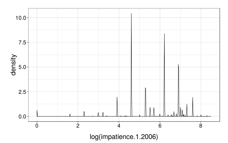
Coding is a subtle issue—we might be able to exploit the fact that many subjects chose a few round answers, rather than treating impatience as having a monotonic effect. A random forest (or rather, bagged decision trees) can do this. Whether it makes senset to recode impatience so that (e.g.) elastic-net regression can exploit this depends on the sample size. Let's see what kinds of sample sizes we're going to get with the many DVs first.

Fitness

h50fl.2.000001.xrnd: how difficult to run a mile xrnd
h50fl.2.000002.xrnd: how difficult to walk several blocks xrnd
h50fl.2.000003.xrnd: how difficult to walk 1 block xrnd
h50fl.2.000004.xrnd: how difficult to sit 2 hours xrnd
h50fl.2.000005.xrnd: how difficult to get up after sitting xrnd
h50fl.2.000006.xrnd: how difficult to climb several flights xrnd
h50fl.2.000007.xrnd: how difficult to climb 1 flight xrnd
h50fl.2.000008.xrnd: how difficult to lift/carry 10 pounds xrnd
h50fl.2.000009.xrnd: how difficult to stoop kneel crouch xrnd
h50fl.2.000010.xrnd: how difficult to pick up dime xrnd
h50fl.2.000011.xrnd: how difficult to raise arms ovr shoulder xrnd
h50fl.2.000012.xrnd: how difficult to pull/push large ojbects xrnd

levels(nlsy$h50fl.2.000012.xrnd)

	x
1	Not at all difficult for you
2	A little difficult
3	Somewhat difficult
4	Very difficult/can't do
5	Don't do

d = rd(d = 2, data.frame(t(sapply(sprintf("h50fl.2.%06d.xrnd", 1:12), function(v) c(
    n = sum(!is.na(nlsy[,v])),
    prop.table(table(nlsy[,v])))))))
colnames(d) = substr(colnames(d), 1, 5)
d

	n	Not.a	A.lit	Somew	Very.	Don.t
h50fl.2.000001.xrnd	4932	0.21	0.14	0.17	0.24	0.24
h50fl.2.000002.xrnd	5003	0.76	0.08	0.07	0.06	0.03
h50fl.2.000003.xrnd	5007	0.88	0.04	0.04	0.03	0.01
h50fl.2.000004.xrnd	5007	0.75	0.08	0.09	0.06	0.01
h50fl.2.000005.xrnd	5006	0.66	0.15	0.13	0.05	0.01
h50fl.2.000006.xrnd	4995	0.60	0.13	0.13	0.11	0.03
h50fl.2.000007.xrnd	5004	0.83	0.06	0.05	0.04	0.01
h50fl.2.000008.xrnd	5000	0.80	0.07	0.07	0.05	0.02
h50fl.2.000009.xrnd	5003	0.64	0.13	0.13	0.09	0.02
h50fl.2.000010.xrnd	5005	0.95	0.02	0.02	0.01	0.00
h50fl.2.000011.xrnd	5006	0.88	0.05	0.05	0.02	0.00
h50fl.2.000012.xrnd	5000	0.78	0.06	0.08	0.06	0.02

On the basis of the table and the item text, let's use:

h50fl.2.000001.xrnd, the difficulty of running a mile, dichotomizing as very hard / can't / don't vs. other options.
h50fl.2.000006.xrnd, the difficulty of climbing several flights of stairs, dichtomizing as not at all vs. other options.
r height in feet 2006
r height in inches 2006
how much does r weigh 2006

nrow(na.omit(nlsy[,qw(q11.10.a.2006, q11.10.b.2006, q11.9.2006)]))

	value
	6923

bmi = 703.06958 * with(nlsy, q11.9.2006 / (q11.10.a.2006 * 12 + q11.10.b.2006)^2)
bmi = bmi[!is.na(bmi)]
ggplot(data.frame(bmi)) +
  geom_densitybw(aes(log(bmi)))

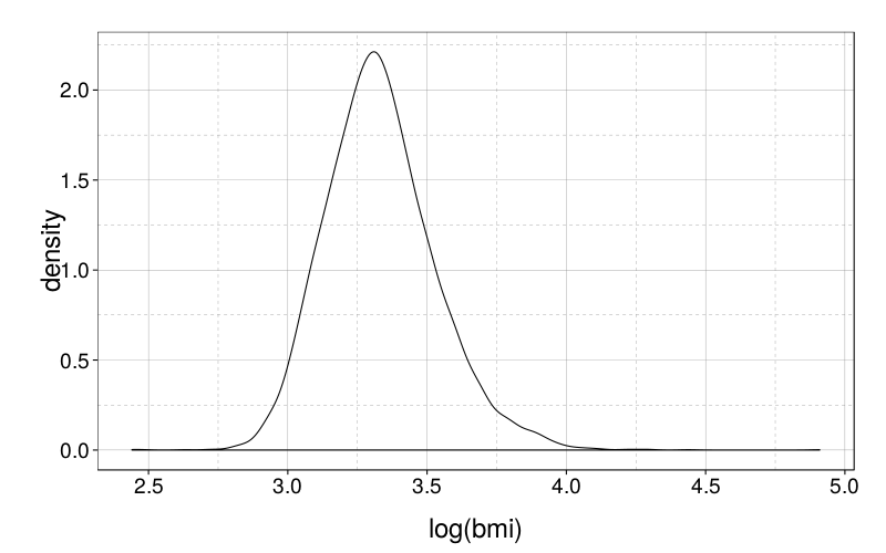
Some of those BMIs are quite extreme, but it's hard to guess which are errors. So let's not remove any data, but evaluate predictions with absolute error rather than squared error.

q11.genhlth.1a.1.2006: freq vigorous exercise 10 > min 2006
q11.genhlth.1a.2.2006: freq vigorous exercise 10 > min 2006
q11.genhlth.1c.1.2006: length vigorous activities 2006
q11.genhlth.1c.2.2006: length vigorous activities 2006
q11.genhlth.2a.1.2006: freq light mod exercise 10 > min 2006
q11.genhlth.2a.2.2006: freq light mod exercise 10 > min 2006
q11.genhlth.2c.1.2006: length light mod activities 10 min 2006
q11.genhlth.2c.2.2006: length light mod activities 10 min 2006
q11.genhlth.3a.1.2006: freq strngth exercise 10 > min 2006
q11.genhlth.3a.2.2006: freq strngth exercise 10 > min 2006

nlsy.exer.vigorous = exercise.freq(nlsy,
   "q11.genhlth.1a.1.2006", "q11.genhlth.1a.2.2006",
   "q11.genhlth.1c.1.2006", "q11.genhlth.1c.2.2006")

c(sum(!is.na(nlsy.exer.vigorous$min.per.year)),
    rd(mean(nlsy.exer.vigorous$min.per.year == 0, na.rm = T)))

	value
	6855 0.319

ggplot(ss(nlsy.exer.vigorous, min.per.year > 0)) +
  geom_densitybw(aes(log(min.per.year))) +
  geom_densitybw(aes(log(min.per.year)), adjust = 10, color = "blue")

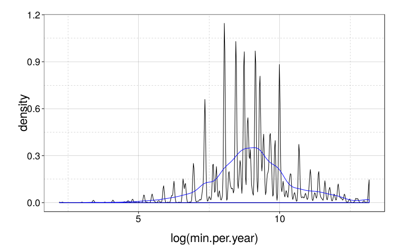
nlsy.exer.light = exercise.freq(nlsy,
   "q11.genhlth.2a.1.2006", "q11.genhlth.2a.2.2006",
   "q11.genhlth.2c.1.2006", "q11.genhlth.2c.2.2006")

c(sum(!is.na(nlsy.exer.light$min.per.year)),
    rd(mean(nlsy.exer.light$min.per.year == 0, na.rm = T)))

	value
	6789 0.262

ggplot(ss(nlsy.exer.light, min.per.year > 0)) +
  geom_densitybw(aes(log(min.per.year))) +
  geom_densitybw(aes(log(min.per.year)), adjust = 10, color = "blue")

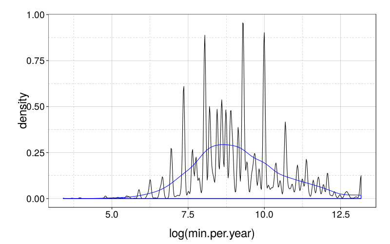
Vigorous and light exercise are probably best predicted with double models that first classify cases as zero or nonzero, and then, in the case of nonzero, estimate the exact number.

nlsy.exer.strength = exercise.freq(nlsy,
   "q11.genhlth.3a.1.2006", "q11.genhlth.3a.2.2006")

c(sum(!is.na(nlsy.exer.strength$freq.per.year)),
    rd(mean(nlsy.exer.strength$freq.per.year == 0, na.rm = T)))

	value
	7097 0.628

Since the frequency for strength exercise isn't far from 50%, let's just predict it dichotomously.

These items are derived:

q11.genhlth.1b.2006: r ever do vigorous activities? 2006
q11.genhlth.2b.2006: r ever do light mod activities? 2006

These are made obsolete for our purposes by the 2006 versions:

q11.9e.2000: freqncy light physical activities? 2000
q11.9f.2000: freq of vigors phys activ/sports? 2000
q11.genhlth.1a.000001.2002: freq vigorous exercise 10 > min 2002
q11.genhlth.1a.000002.2002: freq vigorous exercise 10 > min 2002
q11.genhlth.1c.000001.2002: length vigorous activities 10 min 2002
q11.genhlth.1c.000002.2002: length vigorous activities 10 min 2002
q11.genhlth.2a.000002.2002: freq light mod exercise 10 > min 2002
q11.genhlth.2a.000001.2002: freq light mod exercise 10 > min 2002
q11.genhlth.2c.000001.2002: length light mod activities 10 min 2002
q11.genhlth.2c.000002.2002: length light mod activities 10 min 2002
q11.genhlth.3a.000001.2002: freq strngth exercise 10 > min 2002
q11.genhlth.3a.000002.2002: freq strngth exercise 10 > min 2002

Healthy eating

q11.genhlth.7a.2006: read nutritional info on food 2006

rd(as.data.frame(prop.table(table(nlsy$q11.genhlth.7a.2006, useNA = "always"))))

	Var1	Freq
1	DON'T BUY FOOD	0.010
2	Always	0.301
3	Often	0.180
4	Sometimes	0.192
5	Rarely	0.095
6	Never	0.222
7		0.001

This suggests a trichotomous scheme with the levels "Always or often", "Sometimes", and "Rarely or never". But it would be nice for all my non-numeric DVs to be dichotomous, so let's dichotomize it as Always and Often versus others.

q11.genhlth.7c.1.2008: times ate fast food past 7 days 2008
q11.genhlth.7c.2.2008: time unit eating fast food past 7 days 2008
q11.genhlth.7f.1.2008: times having soft drk or soda past 7 days 2008
q11.genhlth.7f.2.2008: time unit having soft drink or soda past 7 days 2008

fastfood = with(nlsy, ifelse(q11.genhlth.7c.1.2008 == 0,
    0,
    q11.genhlth.7c.1.2008 * ifelse(q11.genhlth.7c.2.2008 == "Per day", 7, 1)))
fastfood = fastfood[!is.na(fastfood)]
fastfood = pmin(fastfood, 3*7)
  # If a subject entered a value greater than 3 times a day every
  # day a week, put it back there.
table(fastfood)

	count
0	2425
1	1849
2	1109
3	631
4	264
5	208
6	39
7	215
8	13
9	7
10	14
12	1
14	24
15	1
20	3
21	20

Since this distribution is very skewed, let's dichotomize it as 0 vs. everything else.

soda = with(nlsy, ifelse(q11.genhlth.7f.1.2008 == 0,
    0,
    q11.genhlth.7f.1.2008 * ifelse(q11.genhlth.7f.2.2008 == "Per day", 7, 1)))
soda = fastfood[!is.na(soda)]
soda = pmin(soda, 3*7)
  # If a subject entered a value greater than 3 times a day every
  # day a week, put it back there.
table(soda)

	count
0	2337
1	1783
2	1062
3	603
4	253
5	199
6	36
7	204
8	13
9	7
10	14
12	1
14	23
20	2
21	19

The same.

Sleep

h50slp.1.xrnd: how much sleep r gets at night on weekdays-hrs xrnd
h50slp.1b.xrnd: how much sleep r gets at night on weekdays-mnts xrnd

ggplot(nlsy) +
    geom_densitybw(aes(h50slp.1.xrnd + h50slp.1b.xrnd/60))

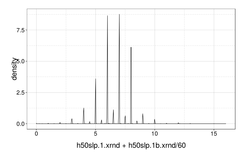
Looks pretty good as is. Let's just use absolute error.

h50slp.2.xrnd: how much sleep r gets at night on weekends-hrs xrnd
h50slp.2b.xrnd: how much sleep r gets at night on weekends-mnts xrnd

with(nlsy, head(rd(sort(
    h50slp.2.xrnd + h50slp.2b.xrnd/60, dec = T)), 20))

	value
	24 24 24 18.3 16 16 15 15 14 14 13 13 13 13 13 12 12 12 12 12

In the weekend data, there are a few rather extreme values. Let's clip them to the maximum of the weekday data, 16 hours.

ggplot(transform(nlsy, x =
    pmin(16, h50slp.2.xrnd + h50slp.2b.xrnd/60))) +
    geom_densitybw(aes(x))

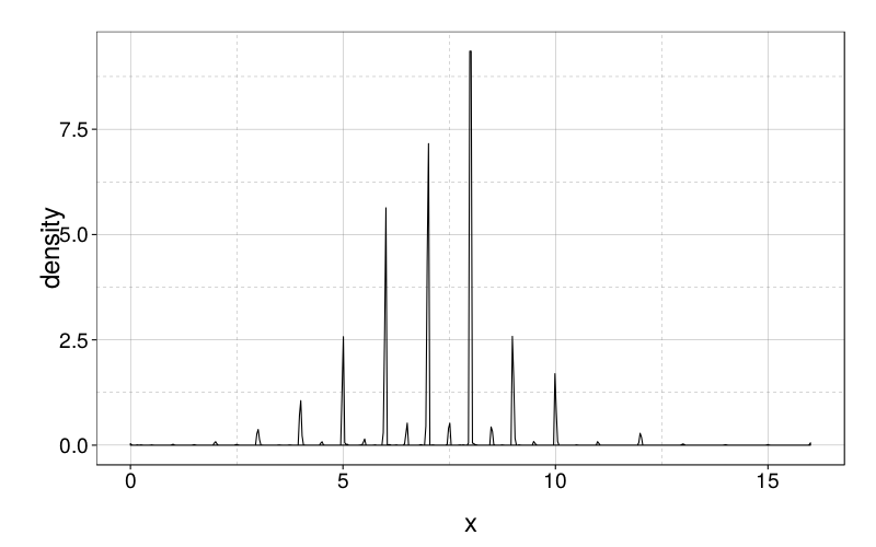
Same as before.

Medical conscientiousness

q11.79.2006: r have health/hosp plan 2006

rd(prop.table(table(useNA = "always", nlsy$q11.79.2006)))

	count
FALSE	0.190
TRUE	0.810
NA	0.001

Looks barely usable.

q11.genhlth.4c.m.000001.2008: med test in past 24 mo - flu shot 2008
q11.genhlth.4c.f.000001.2008: med test in past 24 mo - flu shot 2008

table(useNA = "always", with(nlsy, ifelse(nlsy$sample.sex.1979 == "FEMALE",
    q11.genhlth.4c.f.000001.2008,
    q11.genhlth.4c.m.000001.2008)))

	count
FALSE	4668
TRUE	2184
NA	275

Looks good.

q11.genhlth.4e.m.000001.2008: see/talk to dentist in past 24 months 2008
q11.genhlth.4e.f.000002.2008: see/talk to dentist in past 24 months 2008

table(useNA = "always", with(nlsy, ifelse(nlsy$sample.sex.1979 == "FEMALE",
    q11.genhlth.4e.f.000002.2008,
    q11.genhlth.4e.m.000001.2008)))

	count
FALSE	2273
TRUE	4583
NA	271

Looks good.

q11.genhlth.5a.2.2008: how many times r brush teeth in usual week 2008

table(nlsy$q11.genhlth.5a.2.2008, useNA = "always")

	count
0	15
1	12
2	30
3	24
4	26
5	33
6	10
7	1175
8	21
9	18
10	228
11	11
12	86
13	10
14	3643
15	80
16	48
17	22
18	42
19	5
20	140
21	687
22	1
23	1
24	8
25	22
26	3
27	1
28	75
30	27
35	13
36	1
40	2
42	6
50	3
60	1
63	1
70	10
71	2
73	1
74	1
77	5
100	1
NA	576

Not surprisingly, there are spikes at multiples of 7. I guess the reasonable thing to do is dichtoimze according to whether or not subjects are meeting the usual recommendation of brushing twice a day:

rd(mean(nlsy$q11.genhlth.5a.2.2008 >= 2*7, na.rm = T))

	value
	0.741

q11.genhlth.5a.3.2008: how many times r floss in usual week 2008

table(nlsy$q11.genhlth.5a.3.2008, useNA = "always")

	count
0	1626
1	607
2	573
3	523
4	247
5	287
6	56
7	1742
8	12
9	4
10	83
11	3
12	14
13	2
14	527
15	20
16	5
17	2
18	6
19	1
20	29
21	135
25	4
27	1
28	13
30	4
35	8
40	3
41	1
42	1
50	1
60	1
100	3
NA	583

table(useNA = "always", cut(nlsy$q11.genhlth.5a.3.2008,
    c(0, 1, 7, Inf), right = F))

	count
[0,1)	1626
[1,7)	2293
[7,Inf)	2625
NA	583

We can use the same trichotomy as in the MTurk study. Or, for simplicity, dichotomize according to whether or not the rate attains the usual recommendation of once per week.

Colonoscopies are probably not such a great DV because there isn't a universal recommendation to get them.

q11.genhlth.4c.m.000008.2008: med test in past 24 mo - colonoscopy 2008
q11.genhlth.4c.f.000008.2008: med test in past 24 mo - colonoscopy 2008

Most subjects have teeth, of course.

q11.genhlth.5a.1.2008: r have any of own natural teeth? 2008

Drug use

Tobacco

cig.chk1.2008: r smoked 100 cigarettes 2008
cig.chk2.2008: r ever smoked cigarettes daily 2008
ds.2.2008: smokd at least 100 cigrts in life? 2008
ds.3.1998: r ever smoked daily? 1998
ds.3a.2008: r ever smoked cigarettes daily 2008
ds.4.1998: age when 1st started smoking daily? 1998
ds.5.2008: does r currently smoke daily? 2008
ds.7.2008: # cigarettes smoked per day 2008
q11.genhlth.4b.000003.2006: r asked about smoking at last exam 2006
q11.genhlth.4b.3.2002: asked about smoking at last exam 2002

smoked100 = with(nlsy, cig.chk1.2008 | ds.2.2008)
table(smoked100, useNA = "always")

	count
FALSE	2910
TRUE	3945
NA	272

So we can predict dichotomously whether a subject has smoked 100 cigarettes in their life by 2008.

smokeddaily = with(nlsy, cig.chk2.2008 | ds.3a.2008)
table(smoked100, smokeddaily, useNA = "always")

	FALSE	TRUE	NA
FALSE	0	0	2910
TRUE	207	3738	0
NA	2	2	268

Subjects who hadn't smoked 100 cigarettes weren't asked if they'd ever smoked daily, and among thsoe who had smoked 100 cigarettes, the large majority had smoked daily. So let's ignore the ever-smoked-daily question in favor of ever-smoked-100.

It does seem to make sense to try predict smoking behavior now, though:

table(useNA = "always", ifelse(!smoked100 | !smokeddaily,
   "NOT AT ALL",
    char(nlsy$ds.5.2008)))

	count
DAILY	1464
NOT AT ALL	4988
OCCASIONALLY	403
NA	272

Let's combine OCCASIONALLY and DAILY to get a dichotomous measure of smoking in 2008.

Alcohol

alch.1.1989: alchl-ever had a drnk 89
alch.2.1983: alchl-age start drnk 83
alch.2a.1983: alchl-age start drnk 1 time wk 83
delin.3.1980: ill act # drank alchl past yr <18 80
q12.3.2006: r consumed alcohol in last 30 days? 2006
q12.4.2006: freq of 6 or more drinks at once in last 30 days 2006
q12.5.2006: # of days r drank alcohol last 30 days 2006
q12.6.2006: # of drinks r has on average day 2006
q12.7n.1994: arrested, in police trouble 94 [from drinking]
q12.8.2006: anyone else present during alcohol use questions? 2006

We have some questions from the same year as the impatience questions (2006), so let's use those.

table(nlsy$q12.3.2006, useNA = "always")

	count
FALSE	3338
TRUE	3714
NA	75

This item, of whether the subject drank alcohol in the past 30 days, looks good.

with(nlsy, table(useNA = "always",
    factor(ifelse(q12.3.2006, char(q12.4.2006), "Never in the last 30 days"),
        levels = levels(q12.4.2006))))

	count
Never in the last 30 days	6051
Less often than once a week	480
1 or 2 times per week	335
3 or 4 times per week	99
5 or 6 times per week	46
Everyday	34
NA	82

rd(prop.table(with(nlsy, table(useNA = "always",
    ifelse(q12.3.2006,
      q12.4.2006 != "Never in the last 30 days",
      F)))))

	count
FALSE	0.849
TRUE	0.139
NA	0.012

This gets us a dichotomous measure of heavy drinking. The base rate is low, but we do, after all, have a large sample.

drinks.last.month = with(nlsy,
  ifelse(!q12.3.2006, 0,
  q12.5.2006 * q12.6.2006))
drinks.last.month = drinks.last.month[!is.na(drinks.last.month)]
rd(mean(drinks.last.month == 0))

	value
	0.475

ggplot(data.frame(d = drinks.last.month[drinks.last.month > 0])) +
    geom_bar(aes(log(d), ..ncount..), binwidth = .05) +
    geom_densitybw(aes(log(d)), fill = "blue", alpha = .5, adjust = 15)
#    scale_x_log10()

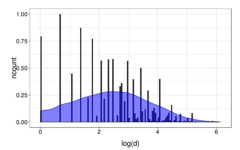
This is probably about the best we can do.

Cannabis

delin.12.1980: ill act smoked marj past yr 80
drug.3.1984: drug month use marj/hash 1st tm 84
ds.8.1998: tot occasion r use marijuana 1998
ds.9.1998: age 1st time used marijuana 1998
ds.10.1998: m-rcnt time used marijuana 1998
ds.11.1998: nmbr times pot past 30 days 1998

table(nlsy$ds.8.1998, useNA = "always")

	count
100 OR MORE TIMES	1039
50 TO 99 TIMES	450
11 TO 49 TIMES	681
6 TO 10 TIMES	481
3 TO 5 TIMES	508
1 OR 2 TIMES	953
NEVER	2550
NA	465

Dichotomizing as NEVER vs. not NEVER looks good.

with(nlsy, rd(prop.table(table(
    ifelse(ds.8.1998 == "NEVER", F,
    ds.10.1998 == "LESS THAN ONE MONTH (30 DAYS) AGO")))))

	count
FALSE	0.944
TRUE	0.056

This measures whether subjects have used cannabis in the past 30 days, but the base rate seems too low.

Nor can we really measure the number of times cannabis was used in the past 30 days conditional on at least one use, because ds.11.1998 is also discretized:

table(nlsy$ds.11.1998, useNA = "ifany")

	count
EVERY DAY	77
5-6 DAYS PER WEEK	32
3-4 DAYS PER WEEK	58
1-2 DAYS PER WEEK	71
LESS OFTEN THAN ONCE A WEEK	133
NA	6756

Cocaine

drug.22.1984: drug use cocaine 84
ds.12.1998: how many occasions used cocaine 1998
ds.13.1998: age 1st time used cocaine 1998
ds.14.1998: m-rcnt time used cocaine 1998
ds.15.1998: occasion used cocaine past 30 days 1998
ds.16.1998: how many occasions used crack 1998
ds.17.1998: age 1st time used crack 1998
ds.18.1998: m-rcnt time used crack 1998
ds.19.1998: occasion used crack past 30 days 1998

table(nlsy$ds.12.1998 != "NEVER", useNA = "ifany")

	count
FALSE	5132
TRUE	1558
NA	437

This is a dichotomous measure of lifetime cocaine use. As in the case of cannabis, this is the most we're going to get.

rd(prop.table(table(nlsy$ds.16.1998 != "NEVER")))

	count
FALSE	0.933
TRUE	0.067

For crack, even the lifetime base rate is quite low.

Other drugs

delin.13.1980: ill act # used drugs past yr 80

table(useNA = "always", nlsy$delin.13.1980 != "NEVER")

	count
FALSE	5514
TRUE	1180
NA	433

This is a dichotomous measure of illegal drug use other than cannabis. In the year before the 1980 interview.

drug.12.1984: drug age 1st use amphtmn/stmlnts 84
ds.27.1998: used stimulants w/o doctor's instr 1998

rd(prop.table(table(useNA = "always", nlsy$ds.27.1998)))

	count
FALSE	0.835
TRUE	0.106
NA	0.058

Borderline. But perhaps worth including for variety.

drug.15.1984: drug age 1st use brbturts/sedtvs 84
drug.18.1984: drug age 1st use trnqlzrs 84
drug.21.1984: drug age 1st use psychdlics 84
drug.25.1984: drug age 1st use heroin 84
drug.31.1984: drug age 1st use inhalants 84
drug.26.1984: drug use other narcotics 84
drug.27.1984: drug #tms use other narcotics 84
drug.28.1984: drug age 1st use other narcotics 84
drug.32.1984: drug use any other drugs 84
drug.33.1984: drug #tms use other drugs 84
drug.34.1984: drug age 1st use other drugs 84

Mostly, the base rates seem to be too low:

rd(mapcols(nlsy[,sprintf("drug.%2d.1984", c(15, 18, 21, 25, 31, 27, 28, 33, 34))],
    function(v) mean(!is.na(v))))

	value
drug.15.1984	0.067
drug.18.1984	0.054
drug.21.1984	0.075
drug.25.1984	0.006
drug.31.1984	0.020
drug.27.1984	0.037
drug.28.1984	0.036
drug.33.1984	0.005
drug.34.1984	0.005

Sexual behavior

mfer.15.1983: male age 1st had intercourse 83
mfer.15.1984: male age 1st had intercourse 84
mfer.15.1985: male age 1st had intercourse 85
ffer.92.1984: f age 1st had sexual intercourse 83
ffer.92.1983: f age 1st had sexual intercourse 84
ffer.92.1985: f age 1st had sexual intercourse 85

age.first.sex = with(nlsy, ifelse(sample.sex.1979 == "FEMALE",
  ifna(ffer.92.1983, ifna(ffer.92.1984, ffer.92.1985)),
  ifna(mfer.15.1983, ifna(mfer.15.1984, mfer.15.1985))))
table(!is.na(age.first.sex))

	count
FALSE	564
TRUE	6563

ggplot(data.frame(x = age.first.sex[!is.na(age.first.sex)])) +
    geom_bar(aes(ordered(x, levels = min(x) : max(x)))) +
    scale_x_discrete(drop = F) +
    no.gridlines()

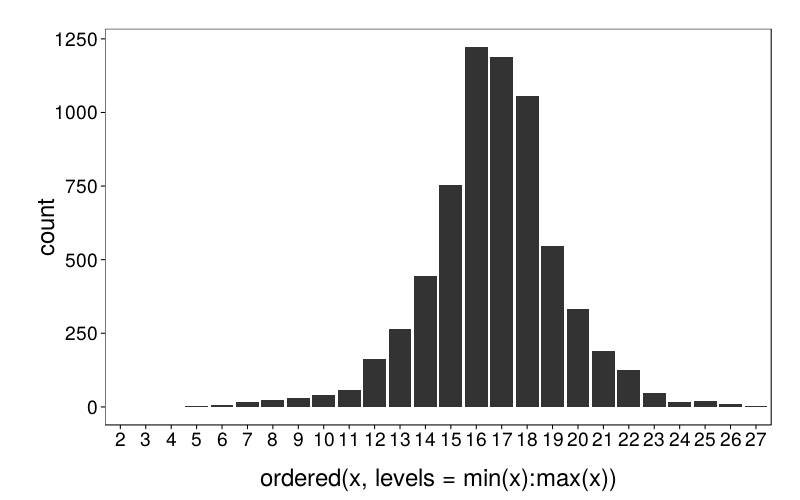
This measures the age of first "sexual intercourse", conditional on having had such by the 1985 interview. Looks good.

For the rest, it isn't really clear what to expect in terms of patience or self-control. The relatively complex way the NLSY measures reproduction and reproductive intentions makes things difficult.

ffer.15.1983: f #tms preg (no live birth lint) 83
ffer.17.1982: f #tms preg b4 birth child#1 82
ffer.23.1982: f #tms preg birth last child 82
mfer.12.1985: male ever had sexual intercourse 85
mfer.13.1983: male had intercourse past month 83
ffer.90.1985: f ever had sexual intercourse 85
ffer.91.1983: f sexual intercourse past mo 83
mfer.26.1985: male #tms intercourse past month 85
mfer.28.1990: male use c-cptn during last mo 90
ffer.92a.1985: f use b-dt yr/1st intercourse 85
ffer.92.m.1985: f mo sexual intercourse 1st time 85
ffer.137.1985: f #tms intercourse past mo 85
ffer.139.1990: f c-cptn during last mo 90
q9.64g.2000: r answer expecting information? 2000
q9.65.000001.2006: contraception meth pill 2006
q9.65.000002.2006: contraception meth condom 2006
q9.65.000003.2006: contraception meth foam 2006
q9.65.000004.2006: contraception meth jelly/cream 2006
q9.65.000005.2006: contraception meth suppstry/insert 2006
q9.65.000006.2006: contraception meth diaphragm 2006
q9.65.000007.2006: contraception meth douching 2006
q9.65.000008.2006: contraception meth iud/coil/loop 2006
q9.65.000009.2000: contraception meth f sterilization 2000
q9.65.000010.2000: contraception meth m sterilization 2000
q9.65.000011.2006: contraception meth family planning 2006
q9.65.000012.2006: contraception meth rhythm 2006
q9.65.000013.2006: contraception meth withdrawal 2006
q9.65.000014.2006: contraception meth sponge 2006
q9.65.000015.2006: contraception meth abstinence 2006
q9.65.000017.2006: contraception meth norplant 2006
q9.65.000018.2004: contraception meth cervical cap 2004
q9.65.000016.2006: contraception meths other 2006
q9.64h.2006: use any contraception dur lst mo? 2006
q9.65.000020.2006: contraception meth hysterectomy 2006
q9.65.000021.2006: contraception meth depo pravara 2006

Divorce

mobg2m.xrnd: mon began 2nd marriage xrnd
yrbg2m.xrnd: year began 2nd marrg xrnd
mobg3m.xrnd: month began 3rd marrg xrnd
yrbg3m.xrnd: year began 3rd marrg xrnd

Counting divorces is too dicey: it seems that variables about numbers of marriages are only derived from changes in marital status reported at each interview.

We could, however, try dichotomizing by the number of subjects who have ever divorced (or separated) at least once.

mar.1.1979: marital status 79
marstat.key.1979: marital status 79
marstat.key.1980: marital status 80
marstat.key.1981: marital status 81
marstat.key.1982: marital status 82
marstat.key.1983: marital status 83
marstat.key.1984: marital status 84
marstat.key.1985: marital status 85
marstat.key.1986: marital status 86
marstat.key.1987: marital status 87
marstat.key.1988: marital status 88
marstat.key.1989: marital status 89
marstat.key.1990: marital status 90
marstat.key.1991: marital status 91
marstat.key.1992: marital status 92
marstat.key.1993: marital status 93
marstat.key.1994: marital status 94
marstat.key.1996: marital status 96
marstat.key.1998: marital status 1998
marstat.key.2000: marital status 2000
marstat.key.2002: marital status 2002
marstat.key.2004: marital status 2004
marstat.key.2006: marital status 2006
marstat.key.2008: marital status 2008
marstat.key.2010: marital status 2010
marstat.key.2012: marital status 2012

table(c(recursive = T, lapply(
    nlsy[,grep("^marstat\\.key", colnames(nlsy), val = T)], levels)))

	count
0: 0 NEVER MARRIED	7
0: NEVER MARRIED	1
1: 1 MARRIED	7
1: MARRIED	1
2: 2 SEPARATED	7
2: SEPARATED	1
3: 3 DIVORCED	7
3: DIVORCED	1
6: 6 WIDOWED	7
6: WIDOWED	1
Divorced	2
DIVORCED	15
Married	2
MARRIED	15
Never Married	2
NEVER MARRIED	15
REMARRIED	14
Separated	2
SEPARATED	15
Widowed	2
WIDOWED	15

So much for consistency in coding. :P

table(useNA = "always", maprows(
    nlsy[,grep("^marstat\\.key", colnames(nlsy), val = T)],
    function(v)
       {v = tolower(char(v))
        any(grepl("divorce", v) | grepl("separ", v))}))

	count
FALSE	3822
TRUE	3305
NA	0

Slightly under half have ever divorced. Sounds about right.

Crime (not drugs)

police.1.1980: stop by police o/than min trafic off 80

rd(prop.table(table(useNA = "always", nlsy$police.1.1980)))

	count
FALSE	0.798
TRUE	0.171
NA	0.031

Looks good.

police.3.1980: ever convicted on ilgl act charges 80
police.3a.1980: times convicted ilgl act excld minor 80
police.3b.1980: age @ time 1st ilgl act conviction 80
police.3e.1980: ever convicted ilgl act adlt court 80

rd(prop.table(table(useNA = "always", nlsy$police.3.1980)))

	count
FALSE	0.922
TRUE	0.047
NA	0.03

Quite a low base rate, but as the only representative of actually committing crime, it's probably worth including anyway.

Income

tnfi.trunc.2006: total net family income 2006

income = nlsy$tnfi.trunc.2006
ggplot(data.frame(v = income[!is.na(income)])) +
    geom_bar(aes(sqrt(v), ..ncount..), binwidth = 2)

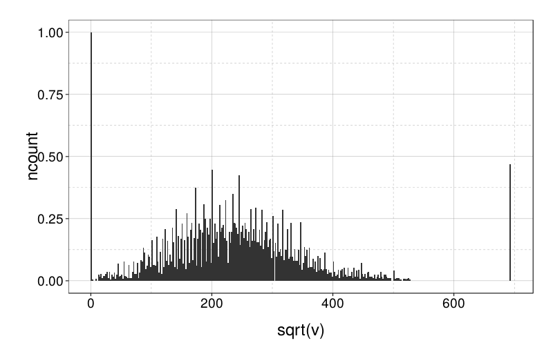
Looks good except for those spikes, which don't comprise much of the data:

rd(mean(nlsy$tnfi.trunc.2006 < 0 | nlsy$tnfi.trunc.2006 > 278500, na.rm = T))

	value
	0.017

Savings

income.21.1982: r/sp have any savings 82
q13.121.2000: any money in savings accounts? 2000
income.35.1988: r/sp set aside money for savings 88
income.35a.trunc.1988: tot amt set aside for savings 87 88

with(nlsy, rd(prop.table(table(useNA = "always", q13.121.2000))))

	count
FALSE	0.264
TRUE	0.665
NA	0.071

The question text here is "Do you (and your spouse) have any money in savings or checking accounts, savings and loan companies, money market funds, credit unions, U.S. savings bonds, individual retirement accounts (IRA or Keogh), or certificates of deposit, common stock, stock options, bonds, mutual funds, rights to an estate or investment trust, or personal loans to others or mortgages you hold (money owed to you by other people)?". It's kind of surprising there are so many FALSE answers. But I'll take it.

q13.123.2000: any money in iras or keough? 2000
q13.123b.2000: any money in tax-defrd plans? 2000
q13.123d.2000: any money in cds,loans,mortg 2000

The first two of these are retirement accounts, which a better indication of deliberately saving money in the long term than, for example, having a checking account. So let's look at those specifically.

with(nlsy, rd(prop.table(table(useNA = "always",
    q13.123.2000 | q13.123b.2000))))

	count
FALSE	0.441
TRUE	0.485
NA	0.074

Let's use these dichotomous variables in preference to amount variables, which, after all, should depend a lot on income and age.

qes1p.10.01.1996: pay pct rs contrib 1st rtrmnt plan 1 96
qes1p.11.01.1996: tim u rs set contrb 1st rtrmnt plan 1 96
qes1p.12.01.1996: set amt rs contrib 1st rtrmnt plan 1 96
qes1p.10.02.1996: pay pct rs contrib 2nd rtrmnt plan 1 96
qes1p.11.02.1996: tim u rs set contrb 2nd rtrmnt plan 1 96
qes1p.12.02.1996: set amt rs contrib 2nd rtrmnt plan 1 96
qes1p.10.03.1996: pay pct rs contrib 3rd rtrmnt plan 1 96
qes1p.11.03.1996: tim u rs set contrb 3rd rtrmnt plan 1 96
qes1p.12.03.1996: set amt rs contrib 3rd rtrmnt plan 1 96
qesp.13.01.01.1998: amt in pnsn/rtrmnt acct now l1,1 1998
qesp.13.01.02.1998: amt in pnsn/rtrmnt acct now l1,2 1998
qesp.13.01.03.1998: amt in pnsn/rtrmnt acct now l1,3 1998
qesp.13.02.01.1998: amt in pnsn/rtrmnt acct now l2,1 1998
qesp.13.02.02.1998: amt in pnsn/rtrmnt acct now l2,2 1998
qesp.13.02.03.1998: amt in pnsn/rtrmnt acct now l2,3 1998
qesp.13.03.01.1998: amt in pnsn/rtrmnt acct now l3,1 1998
qesp.13.03.02.1998: amt in pnsn/rtrmnt acct now l3,2 1998
qesp.13.04.01.1998: amt in pnsn/rtrmnt acct now l4,1 1998
qesp.13.04.02.1998: amt in pnsn/rtrmnt acct now l4,2 1998

These are hypothetical questions:

socsec.2.2004: ss prog or replace with pers ret 2004
socsec.3a.000001.2004: personal acct investments - stocks 2004
socsec.3a.000002.2004: personal acct investments - private bonds 2004
socsec.3a.000003.2004: personal acct investments - govt bonds 2004
socsec.3b.1.2004: any type pers investmts chosen 2004
socsec.3c000001.2004: % of ret acct put into investment 2004
socsec.3c000002.2004: % of ret acct put into investment 2004
socsec.3c000003.2004: % of ret acct put into investment 2004
socsec.4.2004: retirement acct - lump sum or monthly payment 2004

These are better replaced with equivalent questions asked in 1996:

qes1p.10.1.1994: pay pct rs contrib 1st rtrmnt plan 94
qes1p.11.1.1994: tim u rs set contrib 1st rtrmnt plan 94
qes1p.12.1.1994: set amt rs contrib 1st rtrmnt plan 94
qes1p.10.2.1994: pay pct rs contrib 2nd rtrmnt plan 94
qes1p.11.2.1994: tim u rs set contrib 2nd rtrmnt plan 94
qes1p.10.3.1994: pay pct rs contrib 3rd rtrmnt plan 94
qes1p.11.3.1994: tim u rs set contrib 3rd rtrmnt plan 94
qes1p.12.3.1994: set amt rs contrib 3rd rtrmnt plan 94

Debt

ps.1.2008: r miss pay or been late for 5 years 2008

with(nlsy, rd(prop.table(table(useNA = "always", ps.1.2008))))

	count
FALSE	0.755
TRUE	0.204
NA	0.042

Looks good.

debt.1.2008: r-sp has/owes money on credit cards 2008
debt.1a.trunc.2004: tot bal owed on all credit cards 2004
debt.1a.imputed.2008: tot bal owed on all credit cards 2008
debt.1a.2008: tot bal owed on all credit cards 2008
ps.2.2008: # of credit cards owes maximum amt 2008

with(nlsy, rd(prop.table(table(useNA = "always",
   ifelse(debt.1.2008, debt.1a.2008 > 0, F)))))

	count
FALSE	0.492
TRUE	0.435
NA	0.073

Also looks good.

cc.debt = nlsy$debt.1a.2008
cc.debt = cc.debt[!is.na(cc.debt) & cc.debt > 0]
ggplot(data.frame(cc.debt)) +
    geom_bar(aes(log(cc.debt), ..ncount..), binwidth = .1) +
    geom_densitybw(aes(log(cc.debt)), fill = "blue", alpha = .5)

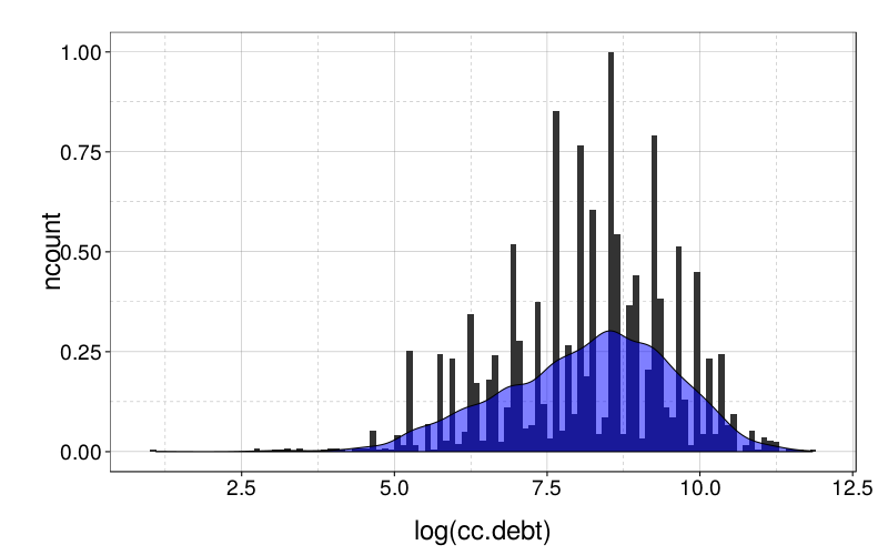
Looks decent.

with(nlsy, rd(prop.table(table(useNA = "always", ps.2.2008 > 0))))

	count
FALSE	0.844
TRUE	0.107
NA	0.049

It's doable.

debt.3.2008: r-sp owes money to oth bus 2008
debt.3a.trunc.2008: tot amt r-sp owes to other bus 2008
debt.3a.2010: tot amt r-sp owes to other bus 2010

with(nlsy, rd(prop.table(table(useNA = "always", debt.3.2008))))

	count
FALSE	0.761
TRUE	0.195
NA	0.044

Looks decent.

debt.4.2008: r-sp ow $1000-more to pers/inst/co 2008
debt.4a.trunc.2008: amt of debt owto oth pers/instit/co 2008
debt.4a.2010: amt of debt owto oth pers/instit/co 2010

with(nlsy, rd(prop.table(table(useNA = "always", debt.4.2008))))

	count
FALSE	0.907
TRUE	0.050
NA	0.043

The base rate's too low.

q13.141.2008: any mony left aft all debts paid? 2008

with(nlsy, rd(prop.table(table(useNA = "always", q13.141.2008))))

	count
Have something left over	0.660
Break even	0.180
Be in debt	0.109
NA	0.052

That middle category is problematic, because given the granularity of assets and debts, there's no way more than a handful of people could truly break even. I expect that people said they would break even because they would roughly break even, and of course, different people should've had different ideas of how close the sum had to be to 0 in order to feel it was close enough. How annoying. I think the only thing to do is to lump the middle category in with "Have something left over", so then we get roughly the dichotomous measure I wanted, of whether subjects owe more than they own.

It's not clear what to expect with regard to student loans, os let's ignore that kind of debt:

debt.2.2008: r-sp resp for make student loan pay 2008
debt.2a.trunc.2004: tot amt r-sp owes on student loans 2004
debt.2c.2008: r-sp make studnt loan pay for child 2008
debt.2d.trunc.2004: amt ow on studnt loans for children 2004
debt.2a.2008: tot amt r-sp owes on student loans 2008
debt.2d.2008: amt ow on studnt loans for children 2008

Only a few subjects got these questions:

debt.1a.sr000001.2008: tot bal owed on all credit cards 2008
debt.1a.sr000002.2008: tot bal owed on all credit cards 2008
debt.1a.uab.a.2008: amt owed on cc accounts > ent amt 2008
debt.1a.uab.b.2008: amt owe on cc accounts > $5k 2008
debt.1a.uab.c.2008: amt owed on credit card accounts > $30k 2008
debt.2a.uab.a.2004: amt ow on studnt loans > ent amt 2004
debt.2a.uab.b.2004: tot amt owed on student loans > 5k 2004
debt.2a.uab.c.2008: tot amt owed on student loans > 30k 2008
debt.2d.uab.a.2008: amt ow on loans for childrn >en amt 2008
debt.3a.uab.a.2008: amt ow to oth bus >ent amt 2008
debt.3a.uab.b.2008: tot amt owed to oth bus >$5k 2008
debt.3a.uab.c.2008: tot amt owed to oth bus >$30k 2008
debt.4a.uab.a.2008: amt of debt ow to oth >ent amt 2008
debt.4a.uab.b.2008: tot amt of debt owed to oth >$5k 2008
debt.4a.uab.c.2008: tot amt of debt owed to oth >$30k 2008

These are procedural codes:

debt.4a.ref.1.2008: r refuse previous inc-ast amounts? 2008
debt.2b.2008: r report bio/adopt/stepchildren 2008

Putting it all together

# Default rules, by data type:
# - logical → binary
# - ordered → ordinal
# - numeric → abs_error

# Evaluate continuous predictions by absolute error, not squared
# error.
# That implies we should use quantile regression instead of
# least squares, so we can predict conditional medians instead of
# condtional means.
# quantreg::rq, quantregForest

isin = function(needle, haystacks)
# Like %in%, but NAs in the first argument return NA, not FALSE.
   ifelse(is.na(needle), NA, needle %in% haystacks)

zero2na = function(v)
    ifelse(v == 0, NA, v)

exer.light = exercise.freq(nlsy,
    "q11.genhlth.2a.1.2006", "q11.genhlth.2a.2.2006",
    "q11.genhlth.2c.1.2006", "q11.genhlth.2c.2.2006")$min.per.year
exer.vig = exercise.freq(nlsy,
    "q11.genhlth.1a.1.2006", "q11.genhlth.1a.2.2006",
    "q11.genhlth.1c.1.2006", "q11.genhlth.1c.2.2006")$min.per.year

nlsy.dvs = with(nlsy, list(

    # Fitness
    hard.to.run.mile = list(
        v = isin(h50fl.2.000001.xrnd,
            c("Very difficult/can't do", "Don't do"))),
    noteasy.to.climb.stairs = list(
        v = h50fl.2.000006.xrnd != "Not at all difficult for you"),
    bmi = list(
        v = 703.06958 * q11.9.2006
            / (q11.10.a.2006 * 12 + q11.10.b.2006)^2,
        trans = log),
    exer.light.ever = list(
        v = exer.light > 0),
    exer.light.min.per.year = list(
        v = zero2na(exer.light),
        trans = log,
        min = 0, max = 365*24*60),
    exer.vig.ever = list(
        v = exer.vig > 0),
    exer.vig.min.per.year = list(
        v = zero2na(exer.vig),
        trans = log,
        min = 0, max = 365*24*60),
    exer.str.ever = list(
        v = !(q11.genhlth.3a.1.2006 == 0 |
            q11.genhlth.3a.2.2006 == "Unable to do this activity")),

    # Healthy eating
    checks.nutrition.often = list(
        v = ifelse(q11.genhlth.7a.2006 == "DON'T BUY FOOD", NA,
            isin(q11.genhlth.7a.2006, qw(Always, Often)))),
#         v = ordered(levels = qw(Often, Sometimes, Rarely),
#             ifelse(q11.genhlth.7a.2006 == "DON'T BUY FOOD", NA,
#             ifelse(isin(q11.genhlth.7a.2006, qw(Always, Often)), "Often",
#             ifelse(isin(q11.genhlth.7a.2006, qw(Rarely, Never)), "Rarely",
#             "Sometimes"))))),
    ate.fast.food.pastweek = list(v =
        q11.genhlth.7c.1.2008 != 0),
    drank.caloric.soda.pastweek = list(v =
        q11.genhlth.7f.1.2008 != 0),

    # Sleep
    sleep.min.weekday = list(
        v = h50slp.1.xrnd*60 + h50slp.1b.xrnd,
        min = 0, max = 16*60),
    sleep.min.weekend = list(
        v = pmin(16*60, h50slp.2.xrnd*60 + h50slp.2b.xrnd),
        min = 0, max = 16*60),

    # Medicine
    health.insurance = list(
        v = q11.79.2006),
    flu.shot.20062008 = list(
        v = ifelse(sample.sex.1979 == "FEMALE",
            q11.genhlth.4c.f.000001.2008,
            q11.genhlth.4c.m.000001.2008)),
    saw.dentist.20062008 = list(
        v = ifelse(nlsy$sample.sex.1979 == "FEMALE",
            q11.genhlth.4e.f.000002.2008,
            q11.genhlth.4e.m.000001.2008)),
    brushes.teeth.twiceweekly = list(
       v = q11.genhlth.5a.2.2008 >= 2*7),
    flosses.weekly = list(
        v = q11.genhlth.5a.3.2008 >= 7),
#        v = ordered(levels = c("<weekly", "<daily", ">=daily"),
#         ifelse(q11.genhlth.5a.3.2008 == 0, "<weekly", 
#             ifelse(nlsy$q11.genhlth.5a.3.2008 < 7, "<daily", ">=daily")))),

    # Drug use
    smoked.100 = list(
        v = cig.chk1.2008 | ds.2.2008),
    smoking.in.2008 = list(
        v = (cig.chk1.2008 | ds.2.2008) &
            (cig.chk2.2008 | ds.3a.2008) &
            isin(ds.5.2008, qw(OCCASIONALLY, DAILY))),
    drank.pastmonth = list(
        v = q12.3.2006),
    drank.heavily.pastmonth = list(
        v = ifelse(!q12.3.2006, F,
           q12.4.2006 != "Never in the last 30 days")),
    drinks.last.month = list(
        v = num(ifelse(!q12.3.2006 | q12.5.2006 == 0 | q12.6.2006 == 0,
            NA,
            q12.5.2006 * q12.6.2006)),
        trans = log),
    used.cannabis.by.1998 = list(
        v = ds.8.1998 != "NEVER"),
    used.cocaine.by.1998 = list(
        v = ds.12.1998 != "NEVER"),
    hard.drugs.in.1980 = list(
        v = delin.13.1980 != "NEVER"),
    used.stims.by.1998 = list(
        v = ds.27.1998),

    # Sexual behavior
    age.first.sex = list(
        v = num(ifelse(sample.sex.1979 == "FEMALE",
          ifna(ffer.92.1983, ifna(ffer.92.1984, ffer.92.1985)),
          ifna(mfer.15.1983, ifna(mfer.15.1984, mfer.15.1985)))),
        min = 0),

    # Divorce
    ever.divorced = list(
        v = maprows(
            nlsy[,grep("^marstat\\.key", colnames(nlsy), val = T)],
            function(v)
               {v = tolower(char(v))
                any(grepl("divorce", v) | grepl("separ", v))})),

    # Crime
    stopped.by.police.1980 = list(
        v = police.1.1980),
    convicted.1980 = list(
        v = police.3.1980),

    # Income
    net.family.income = list(
      v = num(tnfi.trunc.2006), 
      trans = sqrt,
      min = 0,
      max = max(tnfi.trunc.2006, na.rm = T)),

    # Saving
    any.savings = list(
        v = q13.121.2000),
    retirement.account = list(
        v = q13.123.2000 | q13.123b.2000),

    # Debt
    missed.bill.payment = list(
        v = ps.1.2008),
    has.cc.debt = list(
        v = ifelse(debt.1.2008, debt.1a.2008 > 0, F)),
    cc.debt.amnt = list(
        v = num(ifelse(debt.1a.2008 > 0, debt.1a.2008, NA)),
        trans = log),
    maxed.out.cc = list(
        v = ps.2.2008 > 0),
    misc.business.debts = list(
        v = debt.3.2008),
    neg.net.worth = list(
        v = q13.141.2008 == "Be in debt")))

nlsy.dv.classes = sapply(nlsy.dvs,
    function(l) paste(collapse = " ", class(l$v)))

Now for some summaries and checks.

table(nlsy.dv.classes)

	count
logical	31
numeric	9

d = do.call(rbind, lapply(names(nlsy.dvs)[nlsy.dv.classes == "logical"],
    function(name) data.frame(row.names = name,
        n = sum(!is.na(nlsy.dvs[[name]]$v)),
        modal.rate = max(prop.table(table(nlsy.dvs[[name]]$v))),
        mode = mean(nlsy.dvs[[name]]$v, na.rm = T) > .5)))
rd(ordf(d, -modal.rate))

	n	modal.rate	mode
convicted.1980	6910	0.951	FALSE
maxed.out.cc	6775	0.887	FALSE
used.stims.by.1998	6711	0.887	FALSE
neg.net.worth	6759	0.885	FALSE
drank.heavily.pastmonth	7045	0.859	FALSE
hard.drugs.in.1980	6694	0.824	FALSE
stopped.by.police.1980	6907	0.824	FALSE
health.insurance	7123	0.810	TRUE
misc.business.debts	6811	0.796	FALSE
missed.bill.payment	6831	0.787	FALSE
used.cocaine.by.1998	6690	0.767	FALSE
brushes.teeth.twiceweekly	6551	0.741	TRUE
exer.light.ever	6789	0.738	TRUE
smoking.in.2008	6856	0.728	FALSE
any.savings	6618	0.716	TRUE
flu.shot.20062008	6852	0.681	FALSE
exer.vig.ever	6855	0.681	TRUE
saw.dentist.20062008	6856	0.668	TRUE
ate.fast.food.pastweek	6858	0.646	TRUE
exer.str.ever	7097	0.628	FALSE
used.cannabis.by.1998	6662	0.617	TRUE
noteasy.to.climb.stairs	4995	0.604	FALSE
flosses.weekly	6544	0.599	FALSE
drank.caloric.soda.pastweek	6850	0.579	TRUE
smoked.100	6855	0.575	TRUE
ever.divorced	7127	0.536	FALSE
has.cc.debt	6609	0.531	FALSE
drank.pastmonth	7052	0.527	TRUE
hard.to.run.mile	4932	0.524	FALSE
retirement.account	6599	0.523	TRUE
checks.nutrition.often	7053	0.514	FALSE

rd(d = 0, do.call(rbind, lapply(names(nlsy.dvs)[nlsy.dv.classes == "numeric"],
    function(name) data.frame(row.names = name,
        n = sum(!is.na(nlsy.dvs[[name]]$v)),
        t(quantile(nlsy.dvs[[name]]$v, c(0, .025, .25, .5, .75, .975, 1), na.rm = T))))))

	n	X0.	X2.5.	X25.	X50.	X75.	X97.5.	X100.
bmi	6923	11	20	24	27	31	44	136
exer.light.min.per.year	5012	30	720	3120	7800	21900	183900	525600
exer.vig.min.per.year	4667	9	480	3650	7800	18720	175200	525600
sleep.min.weekday	4997	0	240	360	420	480	540	960
sleep.min.weekend	4994	0	240	360	420	480	600	960
drinks.last.month	3691	1	1	4	10	25	120	450
age.first.sex	6563	2	11	15	17	18	22	27
net.family.income	6748	0	0	27000	54975	90212	236932	479983
cc.debt.amnt	3100	3	200	1500	4000	10000	35000	139000

rd(d = 1, do.call(rbind, lapply(names(nlsy.dvs)[
        nlsy.dv.classes == "numeric" & sapply(nlsy.dvs, function(l) "trans" %in% names(l))],
    function(name) data.frame(row.names = name,
        n = sum(!is.na(nlsy.dvs[[name]]$v)),
        t(quantile(nlsy.dvs[[name]]$trans(nlsy.dvs[[name]]$v), c(0, .025, .25, .5, .75, .975, 1), na.rm = T))))))

	n	X0.	X2.5.	X25.	X50.	X75.	X97.5.	X100.
bmi	6923	2.4	3.0	3.2	3.3	3.4	3.8	4.9
exer.light.min.per.year	5012	3.4	6.6	8.0	9.0	10.0	12.1	13.2
exer.vig.min.per.year	4667	2.2	6.2	8.2	9.0	9.8	12.1	13.2
drinks.last.month	3691	0.0	0.0	1.4	2.3	3.2	4.8	6.1
net.family.income	6748	0.0	0.0	164.3	234.5	300.4	486.8	692.8
cc.debt.amnt	3100	1.1	5.3	7.3	8.3	9.2	10.5	11.8

Prediction

Model terms

My first batch of models had only one term each for the two patience items and an interaction. My second will have an additional two dummy variables indicating whether subjects answers 0 on each impatience items, and all possible, identifiable interactions. Starting with the 2⁴ = 16 possible terms, calling the dummy variables d1, d2 and the continuous variables c1, c2:

combs = unlist(rec = F, lapply(0:4, function(i)
    combn(qw(d1, d2, c1, c2), i, simp = F)))
sapply(combs, function(v) paste(v, collapse = " "))

	x
1
2	d1
3	d2
4	c1
5	c2
6	d1 d2
7	d1 c1
8	d1 c2
9	d2 c1
10	d2 c2
11	c1 c2
12	d1 d2 c1
13	d1 d2 c2
14	d1 c1 c2
15	d2 c1 c2
16	d1 d2 c1 c2

we remove all those that contain both d1 and c1, or d2 and c2, to get 9 terms:

combs = combs[sapply(combs, function(l) !(
    ("d1" %in% l && "c1" %in% l) || 
    ("d2" %in% l && "c2" %in% l)))]
sapply(combs, function(v) paste(v, collapse = " "))

	x
1
2	d1
3	d2
4	c1
5	c2
6	d1 d2
7	d1 c2
8	d2 c1
9	c1 c2

Binary DVs

nlsy.predtable.dichotomous = function(iv, formula, brier = F)
    do.call(rbind, lapply((names(nlsy.dvs)[nlsy.dv.classes == "logical"]), function(name)
       {message(name)
        y = nlsy.dvs[[name]]$v
        s = row.names(iv)[which(!is.na(y))]
        y = y[!is.na(y)]
        X = iv[s,]
        judge = function(p, y)
          {if (brier) mean((p - y)^2)
           else       mean((p >= .5) == y)}
        data.frame(row.names = name,
            assoc = local(
               {inpred = predict(glm(formula, cbind(X, y),
                    family = binomial(link = "logit")), type = "response")
                judge(inpred, y)}),
            base.rate = judge(mean(y), y),
            logit = local(
               {pred = crossvalid(X, y, nfold = 10, f = function(train.iv, train.dv, test.iv)
                   {model = glm(formula, cbind(train.iv, y = train.dv),
                        family = binomial(link = "logit"))
                    predict(model, type = "response", newdata = test.iv)})
                judge(pred, y)}),
            rf = (if (brier) NA else local(
               {rf = randomForest(x = X, y = factor(y),
                    ntree = 2000,
                    mtry = ncol(X)) # Since there are only a few predictors.
                1 - tail(rf$err.rate, 1)[1]})))}))

nominal.pred.dichotomous = function(train.iv, train.dv, test.iv)
   {p = tapply(train.dv, train.iv, mean)
    ifna(p[char(test.iv)], mean(train.dv))}

nlsy.predtable.dichotomous.nominaliv = function(iv, brier = F)
    do.call(rbind, lapply((names(nlsy.dvs)[nlsy.dv.classes == "logical"]), function(name)
       {y = nlsy.dvs[[name]]$v
        s = row.names(iv)[which(!is.na(y))]
        y = y[!is.na(y)]
        x = paste(iv[s, "month"], iv[s, "year"])
        # Combine all singleton classes.
        singleton = table(x) == 1
        x = factor(ifelse(singleton[x], "singleton", x))
        judge = function(p, y)
          {if (brier) mean((p - y)^2)
           else       mean((p >= .5) == y)}
        data.frame(row.names = name,
            assoc = judge(nominal.pred.dichotomous(x, y, x), y),
            base.rate = judge(mean(y), y),
            pred = local({
                pred = crossvalid(x, y, nfold = 10, f = nominal.pred.dichotomous)
                judge(pred, y)}))}))

iv.lin = nlsy[,qw(impatience.1.2006, impatience.2.2006)]
colnames(iv.lin) = qw(month, year)
iv.log = ss(select = -c(month, year), transform(iv.lin,
    month0 = month == 0,
    log.month = ifelse(month == 0, 0, log(month)),
    year0 = year == 0,
    log.year = ifelse(year == 0, 0, log(year))))

rd(d = 2, cached(nlsy.predtable.dichotomous(iv.lin,
    y ~ month * year)))

	assoc	base.rate	logit	rf
hard.to.run.mile	0.52	0.52	0.52	0.50
noteasy.to.climb.stairs	0.60	0.60	0.60	0.58
exer.light.ever	0.74	0.74	0.74	0.72
exer.vig.ever	0.68	0.68	0.68	0.67
exer.str.ever	0.63	0.63	0.63	0.60
checks.nutrition.often	0.51	0.51	0.51	0.52
ate.fast.food.pastweek	0.65	0.65	0.65	0.62
drank.caloric.soda.pastweek	0.58	0.58	0.58	0.57
health.insurance	0.81	0.81	0.81	0.80
flu.shot.20062008	0.68	0.68	0.68	0.67
saw.dentist.20062008	0.67	0.67	0.67	0.64
brushes.teeth.twiceweekly	0.74	0.74	0.74	0.73
flosses.weekly	0.60	0.60	0.60	0.58
smoked.100	0.58	0.58	0.58	0.55
smoking.in.2008	0.73	0.73	0.73	0.72
drank.pastmonth	0.53	0.53	0.53	0.55
drank.heavily.pastmonth	0.86	0.86	0.86	0.85
used.cannabis.by.1998	0.62	0.62	0.62	0.61
used.cocaine.by.1998	0.77	0.77	0.77	0.76
hard.drugs.in.1980	0.82	0.82	0.82	0.81
used.stims.by.1998	0.89	0.89	0.89	0.88
ever.divorced	0.54	0.54	0.54	0.54
stopped.by.police.1980	0.82	0.82	0.82	0.82
convicted.1980	0.95	0.95	0.95	0.95
any.savings	0.72	0.72	0.72	0.70
retirement.account	0.53	0.52	0.53	0.56
missed.bill.payment	0.79	0.79	0.79	0.77
has.cc.debt	0.53	0.53	0.53	0.52
maxed.out.cc	0.89	0.89	0.89	0.88
misc.business.debts	0.80	0.80	0.80	0.78
neg.net.worth	0.89	0.89	0.89	0.88

With logged predictors and dummy variables for 0 responses:

rd(d = 6, cached(nlsy.predtable.dichotomous(iv.log,
    y ~ month0 + log.month + year0 + log.year +
        month0:year0 + month0:log.year + year0:log.month + log.month:log.year)))

	assoc	base.rate	logit	rf
hard.to.run.mile	0.537510	0.523723	0.524736	0.493309
noteasy.to.climb.stairs	0.603003	0.603804	0.601602	0.584985
exer.light.ever	0.738253	0.738253	0.737958	0.719399
exer.vig.ever	0.682130	0.680817	0.681400	0.665500
exer.str.ever	0.626744	0.627730	0.625194	0.599690
checks.nutrition.often	0.539345	0.513682	0.539061	0.528569
ate.fast.food.pastweek	0.646398	0.646398	0.645815	0.623360
drank.caloric.soda.pastweek	0.580146	0.579124	0.581606	0.573723
health.insurance	0.809912	0.810192	0.809912	0.802752
flu.shot.20062008	0.681261	0.681261	0.680969	0.664915
saw.dentist.20062008	0.670216	0.668466	0.668174	0.646879
brushes.teeth.twiceweekly	0.740650	0.740650	0.740650	0.724622
flosses.weekly	0.598869	0.598869	0.598258	0.577323
smoked.100	0.575638	0.575492	0.574034	0.550109
smoking.in.2008	0.727246	0.727684	0.727538	0.717182
drank.pastmonth	0.541123	0.526659	0.537294	0.549773
drank.heavily.pastmonth	0.858907	0.858907	0.858907	0.854081
used.cannabis.by.1998	0.616482	0.617232	0.616031	0.607175
used.cocaine.by.1998	0.767115	0.767115	0.767115	0.755904
hard.drugs.in.1980	0.823723	0.823723	0.823723	0.814909
used.stims.by.1998	0.887200	0.887200	0.887200	0.883922
ever.divorced	0.536972	0.536271	0.535008	0.541602
stopped.by.police.1980	0.823657	0.823657	0.823657	0.815694
convicted.1980	0.951230	0.951230	0.951230	0.948915
any.savings	0.715473	0.715624	0.714264	0.704140
retirement.account	0.571450	0.523413	0.570996	0.553569
missed.bill.payment	0.787440	0.787440	0.787440	0.772069
has.cc.debt	0.541232	0.530943	0.540778	0.526555
maxed.out.cc	0.887380	0.887380	0.887380	0.882952
misc.business.debts	0.796212	0.796212	0.796065	0.775510
neg.net.worth	0.885042	0.885190	0.885042	0.879124

With Brier scores:

rd(d = 5, cached(nlsy.predtable.dichotomous(iv.log, brier = T,
    y ~ month0 + log.month + year0 + log.year +
        month0:year0 + month0:log.year + year0:log.month + log.month:log.year)))

[Needs to be regenerated.]

Generally, the logistic regression model achieves predictive accuracy very slightly above the base rate, although not as high as the association, which still isn't high.

Back to percent agreement, but with the IVs fully discretized.

rd(d = 2, nlsy.predtable.dichotomous.nominaliv(iv.lin))

	assoc	base.rate	pred
hard.to.run.mile	0.57	0.52	0.49
noteasy.to.climb.stairs	0.63	0.60	0.58
exer.light.ever	0.75	0.74	0.73
exer.vig.ever	0.69	0.68	0.67
exer.str.ever	0.65	0.63	0.61
checks.nutrition.often	0.58	0.51	0.52
ate.fast.food.pastweek	0.66	0.65	0.63
drank.caloric.soda.pastweek	0.61	0.58	0.58
health.insurance	0.81	0.81	0.80
flu.shot.20062008	0.69	0.68	0.66
saw.dentist.20062008	0.68	0.67	0.65
brushes.teeth.twiceweekly	0.75	0.74	0.73
flosses.weekly	0.62	0.60	0.57
smoked.100	0.60	0.58	0.56
smoking.in.2008	0.74	0.73	0.71
drank.pastmonth	0.59	0.53	0.54
drank.heavily.pastmonth	0.86	0.86	0.85
used.cannabis.by.1998	0.64	0.62	0.60
used.cocaine.by.1998	0.77	0.77	0.75
hard.drugs.in.1980	0.83	0.82	0.81
used.stims.by.1998	0.89	0.89	0.88
ever.divorced	0.58	0.54	0.53
stopped.by.police.1980	0.83	0.82	0.81
convicted.1980	0.95	0.95	0.95
any.savings	0.73	0.72	0.71
retirement.account	0.61	0.52	0.56
missed.bill.payment	0.79	0.79	0.77
has.cc.debt	0.59	0.53	0.54
maxed.out.cc	0.89	0.89	0.88
misc.business.debts	0.80	0.80	0.78
neg.net.worth	0.89	0.89	0.88

The model generally overfits, even though the increase from the base rate to association is still small.

Continuous DVs

nlsy.predtable.cont = function(iv, formula)
    do.call(rbind, lapply(names(nlsy.dvs)[nlsy.dv.classes == "numeric"], function(name)
       {message(name)
        l = nlsy.dvs[[name]]
        y = l$v
        s = row.names(iv)[which(!is.na(y))]
        y = y[!is.na(y)]
        X = iv[s,]
        trans = identity
        untrans = identity
        if ("trans" %in% names(l))
           {trans = l$trans
            if (identical(trans, log))
                untrans = exp
            else if (identical(trans, sqrt))
                untrans = function(v) v^2
            else
                stop()}
        y.min = (if ("min" %in% names(l)) l$min
            else -Inf)
        y.max = (if ("max" %in% names(l)) l$max
            else Inf)
        digest.pred = function(y.pred)
            pmin(y.max, pmax(y.min, untrans(y.pred)))
        data.frame(row.names = name,
            cor.m = cor(X[,(if ("log.month" %in% colnames(X)) "log.month" else "month")], y),
            cor.y = cor(X[,(if ("log.year" %in% colnames(X)) "log.year" else "year")], y),
            assoc = local(
               {inpred = digest.pred(predict(
                    rq(formula, cbind(X, y = trans(y)),
                    tau = .5)))
                mean(abs(inpred - y))}),
            mad = mean(abs(y - median(y))),
            qr = local(
               {pred = digest.pred(crossvalid(X, trans(y), nfold = 10, f = function(train.iv, train.dv, test.iv)
                   {model = rq(formula, cbind(train.iv, y = train.dv),
                        tau = .5)
                    predict(model, newdata = test.iv)}))
                mean(abs(pred - y))}),
            rf = local(
               {rf = quantregForest(x = X, y = trans(y),
                    mtry = ncol(X)) # Since there are only a few predictors.
                pred = digest.pred(predict(rf, quantiles = .5))
                mean(abs(pred - y))}))}))

nominal.pred.cont = function(train.iv, train.dv, test.iv)
   {p = tapply(train.dv, train.iv, median)
    ifna(p[char(test.iv)], median(train.dv))}

nlsy.predtable.cont.nominaliv = function(iv)
    do.call(rbind, lapply(names(nlsy.dvs)[nlsy.dv.classes == "numeric"], function(name)
       {l = nlsy.dvs[[name]]
        y = l$v
        s = row.names(iv)[which(!is.na(y))]
        y = y[!is.na(y)]
        x = paste(iv[s, "month"], iv[s, "year"])
        # Combine all singleton classes.
        singleton = table(x) == 1
        x = factor(ifelse(singleton[x], "singleton", x))
        trans = identity
        untrans = identity
        if ("trans" %in% names(l))
           {trans = l$trans
            if (identical(trans, log))
                untrans = exp
            else if (identical(trans, sqrt))
                untrans = function(v) v^2
            else
                stop()}
        y.min = (if ("min" %in% names(l)) l$min
            else -Inf)
        y.max = (if ("max" %in% names(l)) l$max
            else Inf)
        digest.pred = function(y.pred)
            pmin(y.max, pmax(y.min, untrans(y.pred)))
        data.frame(row.names = name,
            assoc = mean(abs(digest.pred(nominal.pred.cont(x, trans(y), x)) - y)),
            mad = mean(abs(y - median(y))),
            pred = local({
                pred = digest.pred(crossvalid(x, trans(y), nfold = 10, f = nominal.pred.cont))
                mean(abs(pred - y))}))}))

rd(d = 2, cached(nlsy.predtable.cont(iv.lin,
    y ~ month * year)))

	cor.m	cor.y	assoc	mad	qr	rf
bmi	0.00	0.01	4.42	4.43	4.43	4.64
exer.light.min.per.year	-0.01	-0.01	25938.93	25940.94	25948.50	26780.61
exer.vig.min.per.year	0.00	0.01	22186.08	22205.79	22238.68	22968.64
sleep.min.weekday	0.01	0.02	63.29	63.32	63.37	66.40
sleep.min.weekend	-0.02	0.00	73.62	73.66	73.96	75.88
drinks.last.month	0.00	-0.01	17.92	17.92	18.12	18.83
age.first.sex	-0.01	-0.01	1.91	1.91	1.91	1.97
net.family.income	-0.01	-0.01	44124.58	44145.32	44206.65	44475.98
cc.debt.amnt	-0.02	-0.01	5969.76	5972.24	5973.77	6299.73

The correlations are remarkably close to 0.

With logged predictors and dummy variables for 0 responses:

rd(d = 2, cached(nlsy.predtable.cont(iv.log,
    y ~ month0 + log.month + year0 + log.year +
        month0:year0 + month0:log.year + year0:log.month + log.month:log.year)))

	cor.m	cor.y	assoc	mad	qr	rf
bmi	0.04	0.03	4.41	4.43	4.41	4.65
exer.light.min.per.year	-0.01	-0.03	25921.10	25940.94	25952.80	26637.90
exer.vig.min.per.year	-0.01	-0.02	22173.85	22205.79	22196.01	22958.10
sleep.min.weekday	0.01	0.02	63.18	63.32	63.47	66.99
sleep.min.weekend	0.04	0.04	73.18	73.66	73.36	76.47
drinks.last.month	-0.04	-0.03	17.91	17.92	17.94	18.85
age.first.sex	-0.05	-0.03	1.91	1.91	1.92	1.98
net.family.income	-0.07	-0.03	43151.85	44145.32	43242.16	44292.69
cc.debt.amnt	-0.04	-0.01	5961.44	5972.24	5984.10	6257.58

rd(d = 2, nlsy.predtable.cont.nominaliv(iv.lin))

	assoc	mad	pred
bmi	4.26	4.43	4.56
exer.light.min.per.year	25427.31	25940.94	26801.83
exer.vig.min.per.year	21730.30	22205.79	23838.04
sleep.min.weekday	60.37	63.32	66.47
sleep.min.weekend	69.09	73.66	76.68
drinks.last.month	17.34	17.92	18.87
age.first.sex	1.83	1.91	1.99
net.family.income	40976.40	44145.32	44212.97
cc.debt.amnt	5715.25	5972.24	6254.13

The model generally overfits, even though the increase from the base rate to association is still small.

p-values

Dichotomous criterion variables:

ps = t(sapply(nlsy.dvs[nlsy.dv.classes == "logical"], function(l) c(
    month = wilcox.test(iv.lin$month ~ l$v)$p.value,
    year = wilcox.test(iv.lin$year ~ l$v)$p.value)))
c(
   "comparisons" = length(ps),
   "p < .05"     = sum(ps < .05),
   "p < .05/comp" = sum(ps < .05/length(ps)))

	value
comparisons	62
p < .05	45
p < .05/comp	30

Continuous criterion variables:

ps = t(sapply(nlsy.dvs[nlsy.dv.classes == "numeric"], function(l) c(
    month = cor.test(iv.lin$month, l$v, method = "kendall")$p.value,
    year = cor.test(iv.lin$year, l$v, method = "kendall")$p.value)))
c(
   "comparisons" = length(ps),
   "p < .05"     = sum(ps < .05),
   "p < .05/comp" = sum(ps < .05/length(ps)))

	value
comparisons	18
p < .05	7
p < .05/comp	7

References

Beck, R. C., & Triplett, M. F. (2009). Test–retest reliability of a group-administered paper–pencil measure of delay discounting. Experimental and Clinical Psychopharmacology, 17, 345–355. doi:10.1037/a0017078

Chabris, C. F., Laibson, D., Morris, C. L., Schuldt, J. P., & Taubinsky, D. (2008). Individual laboratory-measured discount rates predict field behavior. Journal of Risk and Uncertainty, 37(2, 3), 237–269. doi:10.1007/s11166-008-9053-x

de Gruijter, D. N. M., & van der Kamp, L. J. T. (2008). Statistical test theory for the behavioral sciences. Boca Raton, FL: CRC. ISBN 978-1-58488-958-8.

Harinck, F., Van Dijk, E., Van Beest, I., & Mersmann, P. (2007). When gains loom larger than losses: Reversed loss aversion for small amounts of money. Psychological Science, 18(12), 1099–1105. doi:10.1111/j.1467-9280.2007.02031.x

Horstein, M. (1963). Sequential transmission using noiseless feedback. IEEE Transactions on Information Theory, 9(3), 136–143. doi:10.1109/TIT.1963.1057832

Kirby, K. N. (2009). One-year temporal stability of delay-discount rates. Psychonomic Bulletin and Review, 16(3), 457–462. doi:10.3758/PBR.16.3.457

Kirby, K. N., Petry, N. M., & Bickel, W. K. (1999). Heroin addicts have higher discount rates for delayed rewards than non-drug-using controls. Journal of Experimental Psychology: General, 128(1), 78–87. doi:10.1037/0096-3445.128.1.78

Madden, G. J., Petry, N. M., Badger, G. J., & Bickel, W. K. (1997). Impulsive and self-control choices in opioid-dependent patients and non-drug-using control participants: Drug and monetary rewards. Experimental and Clinical Psychopharmacology, 5(3), 256–262. doi:10.1037/1064-1297.5.3.256

Sayman, S., & Öncüler, A. (2009). An investigation of time inconsistency. Management Science, 55(3), 470–482. doi:10.1287/mnsc.1080.0942

Schuerger, J. M., Tait, E., & Tavernelli, M. (1982). Temporal stability of personality by questionnaire. Journal of Personality and Social Psychology, 43(1), 176–182. doi:10.1037/0022-3514.43.1.176

Smith, C. L., & Hantula, D. A. (2008). Methodological considerations in the study of delay discounting in intertemporal choice: A comparison of tasks and modes. Behavior Research Methods, 40(4), 940–953. doi:10.3758/BRM.40.4.940

Sutter, M., Kochaer, M. G., Rützler, D., & Trautmann, S. T. (2010). Impatience and uncertainty: Experimental decisions predict adolescents' field behavior (Discussion Paper No. 5404). Institute for the Study of Labor. Retrieved from http://ftp.iza.org/dp5404.pdf

van der Linden, W. J., & Glas, C. A. W. (Eds.). (2010). Elements of adaptive testing. New York, NY: Springer. ISBN 978-0-387-85459-5.

Waeber, R. (2013). Probabilistic bisection search for stochastic root-finding (PhD thesis). Cornell University. Retrieved from http://people.orie.cornell.edu/shane/theses/ThesisRolfWaeber.pdf

Weber, B. J., & Chapman, G. B. (2005). Playing for peanuts: Why is risk seeking more common for low-stakes gambles? Organizational Behavior and Human Decision Processes, 97(1), 31–46. doi:10.1016/j.obhdp.2005.03.001

Wulfert, E., Block, J. A., Ana, E. S., Rodriguez, M. L., & Colsman, M. (2002). Delay of gratification: Impulsive choices and problem behaviors in early and late adolescence. Journal of Personality, 70(4), 533–552. doi:10.1111/1467-6494.05013