The unpredictable Buridan's ass: Failure to predict decisions in a trivial decision-making task
Created 14 Feb 2021 • Last modified 5 Oct 2021
In order to better examine seemingly unpredictable variation that appears in decision-making studies, I had people choose between two options that had no features or consequences to distinguish them. 100 users of Mechanical Turk completed 200 binary choices, and I examined the accuracy with which statistical models could predict the choices. Across three different conceptualizations of the prediction problem and a variety of models ranging from logistic regression to neural networks, I obtained at best modest predictive accuracy. Predicting trivial choices may actually be more difficult than predicting meaningful choices. These strongly negative results appear to place limits on the predictability of human behavior.
This paper can be found at PsyArXiv with doi:10.31234/osf.io/qu39a.
Introduction
Social scientists use the word "predict" a lot, but there's been relatively little attention to the problem of predicting individual units of human behavior and checking the accuracy of those predictions (see Arfer, 2016, for a detailed discussion). This issue is related to how statistics in general has emphasized unobservable population features, such as the mean, over predictive accuracy (Geisser, 1993), with machine learning coming to fill this niche in more recent history. I've argued that prediction deserves more attention for the sake of both basic and applied social science (Arfer, 2016). I'm particularly interested in the prediction of decisions.
In one of my first papers (Arfer & Luhmann, 2015), I checked the predictive accuracy of 9 statistical models in a simple laboratory intertemporal-choice task. Several of the models obtained the apparent ceiling of 85% accuracy, which was a good improvement over the base rate of 68%. But I wondered why even sophisticated models couldn't seem to reach 90%, 95%, or 100% accuracy. Whence this seemingly unpredictable variation? How could it be mastered? Subsequent studies (Arfer & Luhmann, 2017; Arfer, 2016) showed that even improvements of the kind I got in Arfer and Luhmann (2015) may not be so easy to get in applied contexts, when trying to predict behavior of real consequence. Perhaps if we learned to predict that leftover variation that appears even in simple decisions, we could learn something about human decision-making with which we could tackle these applied problems.
In the pursuit of simplicity, consider trivial decisions: situations where you can make a decision, but your choice doesn't matter. A classic example is the version of the thought experiment called Buridan's ass in which the donkey is hungry and is midway between two identical bales of hay. The donkey, not being an intellectual, has no trouble deciding which way to go, but how can we predict its choice? In typical decision-making studies, such as studies of intertemporal choice or risky choice, there are meaningful features of the options, such as the size of a reward, that decision-makers use to make their choice. In a trivial decision, there are no such features, so all variation in choices must be unrelated to features—and perhaps of the same kind that led to the 85% ceiling in Arfer and Luhmann (2015). We must resort to superficial aspects of the scenario, such as the order in which options are presented, in order to predict decisions without consulting out-of-task data (such as the subject's gender, or a personality test).
The question of predicting trivial decisions is closely related to the question of how capable humans are of behaving randomly. The latter has gotten a fair amount of attention. Hagelbarger (1956) is an early example of a computer to predict binary choices one at a time in a competitive context. A human makes choices and sees the computer's predictions, while trying to pick the opposite of what it will guess. Merill (2018) is a modern implementation of a similar idea. In a non-competitive version of this method, in which predictve models are trained and tested after all the data was collected, Shteingart and Loewenstein (2016) obtained about 60% accuracy with logistic regression. Broadly, the literature indicates that people fail to produce sequences that pass stringent tests of randomness (Nickerson, 2002; Nickerson & Butler, 2009), although the tests and instructions used matter (Nickerson, 2002) and with practice, people (e.g., Delogu et al., 2020) as well as animals (e.g., Nergaard & Holth, 2020) can learn to produce better random numbers.
Similar to these experiments on random-number generation, I sought in this study to predict trivial decisions. I didn't ask subjects to try to make random choices; instead, I just told them to "choose whichever you like". I had each subject complete 200 trials, with the idea of using the first 100 for training predictive models and the second 100 for testing. I hoped to achieve something like 95% or 100% accuracy in this maximally simple situation in which there are no substantive features to model. I considered more complex models than are typically applied to experiments of random-number generation, with the idea that they might succeed where previous models fell short of high accuracy.
Data collection
The data was collected from 101 users of Mechanical Turk in 2019. One subject, the first, is omitted from all analyses because I accidentally gave them a pilot version of the task; all other subjects are included.
The task was described to prospective subjects thus: "Make some simple decisions. The task takes about 3 minutes." Subjects were required to live in the US and have at least 90% of their previous Mechanical Turk assignments approved. They were given up to 10 minutes to complete the task and were paid 0.75 USD. Given the actual time subjects took for the entire task, including the consent form, this resulted in a median hourly wage of $12.86 (range $4.56 to $45.76). The consent form described the procedure thus: "If you decide to be in this study, your part will involve pressing keys on your device's keyboard to indicate which of various options you prefer."
During the task, subjects saw these instructions on screen:
To complete this task, just make a bunch of decisions.
There are two options to choose from. Nothing special happens when you make a choice, so choose whichever you like.
Press the "f" key to choose the first option, or the "j" key to choose the second.
I chose the "f" and "j" keys for their centrality on QWERTY keyboards. The subjects' choices were encoded such that the first option is regarded as true or the number 1, and the second option as false or the number 0.
There were 200 trials; that is, the subject had to press one of the two keys 200 times. A counter labeled "Trials left" was displayed. There was no visible log of which choices the subject had made. There was also no delay imposed between trials. But the task was programmed such that subjects had to make a separate keypress for each trial, instead of just holding down a key.
I didn't collect any demographic information about the subjects.
Data analysis
Deidentified raw data, task code, analysis code, and a research notebook can be found at http://arfer.net/projects/donkey.
Descriptive information
Figure 1 shows the distribution of choices. Overall, subjects chose truly in 10,240 out of 20,000 trials (51%). This base rate near 50% is helpful for the purposes of this study, since it provides a lot of room for improvement by predictive methods.
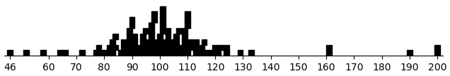
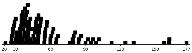
Figure 2 shows the distribution of per-subject sums of response times, omitting the first trial, on which subjects presumably read the instructions. The mean is 58.8 s, so the mean of the individual per-trial response times, again omitting the first trial, is 296 ms; the median is 179 ms. Thus, overall, subjects decided quickly.
Half splits
My first models used a within-subjects approach, in which models were trained and tested on one subject at a time. Each model was trained on the first 100 trials, and its predictions on the latter 100 trials were assessed. The accuracy for each subject is defined as the number of test trials for which the predicted choice equals the observed choice. Throughout this paper, I focus on traditional classification-style measures of accuracy instead of probabilistic classification so that pure classifiers (such as nearest-neighbors classifiers) can be directly compared to models capable of predicting probabilities (such as logistic regression).
The first section of Table 1 shows the quartiles of per-subject accuracies for each model. For comparison, it also includes the quartiles of per-subject base rates, which are computed for each subject as simply the number of true choices or the number of false choices, whichever is greater. In general, the accuracies are about equal to or worse than the base rates, indicating very poor predictive accuracy. Three models are shown:
TrialNumbersis based on logistic regression with a ridge penalty. There are eight predictors, defined as and then standardized, where n is the trial number (counting the first training trial as 0 and the first test trial as 100), and a mod b represents the remainder after division of a by b. The penalty size is chosen per subject with tenfold cross-validation (CV).RunLengthsis a regression model of the same type, but with different predictors, namely (j, k, j2, k2, p), where j is the number of true choices made by this subject so far, k is the number of false choices, and p is 1 if the last choice was true and 0 otherwise (including on trial 0). j and k are reset whenever a choice of the opposite kind is made, so the predictors are determined entirely by the previous trial and how many times that same choice was made in consecutive previous trials. When the previous trial was not observed, j, k, and p are set based on the model's own prediction.SuperMarkovresembles a Markov chain, as its name suggests. It assumes that each choice is a probabilistic function of the n-tuple formed of the previous n choices, where n is a hyperparameter varying from 2 to 5. The prediction is true when the observed choices for the n-tuple were more often true than false, false when they were more often false than true, and the modal choice in case of ties. For each subject, I report the greatest accuracy across values of n.
| Model | Q1 | Median | Q3 |
|---|---|---|---|
| Split-half | |||
| (Base rate) | 51 | 56 | 62 |
TrialNumbers |
48 | 52 | 59 |
RunLengths |
48 | 50 | 54 |
SuperMarkov |
50 | 54 | 64 |
| Interpolation | |||
Trivial |
52 | 55 | 58 |
Cubic |
48 | 54 | 60 |
CubicMod |
53 | 57 | 65 |
KNN |
48 | 58 | 70 |
XGBoost |
54 | 58 | 69 |
Interpolation
There are two ways in which the half-split form of this problem may be especially difficult. If a model is based on trial numbers, it's trained on inputs 0 to 99 and then tested on inputs greater than 99. Thus, the training process places few constraints on the model's behavior for the inputs on which it's tested, and it's forced to extrapolate. On the other hand, an autoregressive kind of model, in which the choice for one trial depends on the choices for previous trials, is fragile, because a bad prediction for trial 102 can impair performance for all 97 remaining trials.
To avoid these issues, I assessed another batch of models in an interpolative fashion, with tenfold CV. The CV folds are chosen randomly for different subjects, but for a given subject, all models use the same folds. This setup resembles Arfer and Luhmann (2015).
The second section of Table 1 shows the resulting accuracies; each is divided by 2 for easier reading, since accuracy in predicting all 200 test trials is now checked. Here, comparison numbers are provided by the model Trivial, which is assessed in the same way as the other models, but works by simply predicting the modal choice in its training set. There is some improvement over Trivial, but not much. Four nontrivial models are shown:
Cubicis an unpenalized logistic-regression model with predictors computed as (n, n2, n3) and then standardized, where n is the trial number.CubicModresemblesTrialNumbers. It's a logistic-regression model with a ridge penalty and predictors (n, n2, n3, n mod 2, n mod 3). The penalty size is chosen per subject with nested tenfold CV.KNNis a k-nearest-neighbors model with one predictor, n. k ranges from 1 to 10 and is chosen with nested CV.XGBoostis an extreme gradient-boosting model (Chen & Guestrin, 2016) with n as the only predictor. The model uses a hinge objective and 250 trees. Five hyperparameters (learning_rate,gamma,reg_lambda,reg_alpha,max_depth) are allowed to vary; I randomly selected a set of 50 hyperparameter vectors, then tested them per subject with nested CV.
Hierarchy
The interpolative form of the problem, while not as difficult as the half-split approach, still doesn't allow models to learn things about human behavior from one subject and apply that knowledge to other subjects. With each new subject, the model starts from square one. For a final batch of models, I switched to a between-subjects CV approach. Here I treat each subject's first 100 trials as predictors for that subject and the latter 100 trials as dependent variables, modeling each of these test trials separately. (For simplicity, I only actually test 3 of the 100 test trials.) In some models, I also provide the response times (RTs) for the first 100 trials as additional predictors, although I neither test nor train on RTs for the test trials. The models use no predictors beyond the 100 training choices and 100 training RTs.
Table 2 shows base rates and accuracies for 3 of the test trials. For trials 100 and 101, the first two test trials, we see some improvement over the base rate. Still, the accuracies are far short of 100 or 98, topping out at 73 against a base rate of 50. For trial 150, which is 50 trials after the last training trial, performance is less impressive yet, topping out at 56 against a base rate of 55. Hence, while these between-subjects models may have some predictive ability, there remains quite a lot of unpredictable variation. Six models are shown:
OneColis a simplistic model that finds the single most predictive trial of the 100 training trials for the given test trial, and uses only that trial to make its predictions.Regressionis a logistic-regression model with a lasso penalty. Penalty sizes were set by hand per test trial.KNNis a 3-nearest-neighbors model. I set k = 3 by hand.NeuralNetworkis a neural network with one layer of hidden nodes. There are 100 hidden nodes for the models without RTs and 200 hidden nodes for the models with them. The hidden nodes use a hyperbolic-tangent activation function, regularized with a manually sized lasso penalty. The output node uses a sigmoid activation function. The network was fit with TensorFlow's RMSprop optimizer and cross-entropy loss.
| Model | RTs | 100 | 101 | 150 |
|---|---|---|---|---|
| (Base rate) | 55 | 50 | 55 | |
OneCol |
False | 68 | 77 | 52 |
Regression |
False | 66 | 73 | 53 |
Regression |
True | 66 | 73 | 53 |
3NN |
False | 61 | 57 | 56 |
3NN |
True | 57 | 60 | 55 |
NeuralNetwork |
False | 60 | 68 | 55 |
NeuralNetwork |
True | 61 | 70 | 55 |
Discussion
In this task, with this population, choices are not entirely unpredictable. Nevertheless, it's striking how far short I fell of the goal of 95% or 100% accuracy, considering both small, simple models and big, fancy models. Even the performances I obtained are in some cases likely overestimated because I was sloppy with hyperparameters, setting them manually instead of with nested CV or another method to avoid overfitting; by that point, my goal was merely to get a ceiling and confirm my hunch that the kind of accuracy I was looking for wasn't going to happen. The models of Arfer and Luhmann (2015) did much better, suggesting that decisions without meaningful features are actually harder, not easier, to predict.
I'm not sure what to make of this. Here are some possibilities, not all of which are mutually exclusive:
- The basic idea behind this study was sound, but my sample wasn't big enough. After all, in the hierarchy case, I had only 100 subjects for a dataset with 100 or 200 predictors. The gap between the kind of accuracy I was looking for and the accuracy I got makes me think that a twofold or even tenfold increase in sample size probably wouldn't have solved the problem. Much bigger samples, say tens of thousands of people, could more feasibly have made the difference, but they'd be expensive, even at the very modest rate I paid these subjects.
- These choices are predictable given more information about the subjects, such as their gender, their complete history of choices in similar situations throughout their life, or a high-resolution scan of their brain. I'm skeptical that the more feasibly collected information of this kind would be helpful considering some of my previous studies (Arfer & Luhmann, 2017; Arfer, 2016). The best predictors of behavior seems to generally be other behavior of the same kind. It's just that, as in this study, sometimes the best predictors aren't good enough.
- People are simply capable of behaving unpredictably. This brings to mind the old question of whether the universe itself is deterministic or probabilistic, but this metaphysical issue isn't as important as it might sound, since probabilistic systems can be highly predictable whereas deterministic systems can defy predictability with e.g. chaos (Hoefer, 2016). Some behaviorists have argued that variation itself is a reinforcable dimension of behavior (Nergaard & Holth, 2020). Perhaps humans as well as other animals have a specifically evolved ability to generate random numbers, to help with things like choosing a foraging location while minimizing competition or predictability by predators, even if this ability is imperfect. This is an ugly possibility to consider for any scientist who's interested in the prediction of behavior, but here we are.
- People would behave differently, and more predictably, in a more Buridan's ass-like situation in which, although the options are still equivalent, the outcome is consequential (avoiding starvation, in the donkey's case).
I didn't specifically ask subjects not to use a randomization device, like a coin. This was probably a mistake. Some may have used a randomization device. This said, the quick response times suggest that it wasn't common. 179 ms doesn't seem like enough time to flip a coin and read and input the result.
Incidentally, it's perhaps surprising that the left-hand option was more popular overall. Past research suggests that people associate goodness with the direction of their dominant hand and badness with the direction of their off-hand (Casasanto & Chrysikou, 2011; Casasanto & Henetz, 2012), an idea applied specifically to QWERTY keyboards by Jasmin and Casasanto (2012), and most people are right-handed.
References
Arfer, K. B. (2016). Predicting outcomes of interventions to increase social competence in children and adolescents (PhD thesis). State University of New York at Stony Brook. Retrieved from http://arfer.net/projects/pelt/paper
Arfer, K. B., & Luhmann, C. C. (2015). The predictive accuracy of intertemporal-choice models. British Journal of Mathematical and Statistical Psychology, 68(2), 326–341. doi:10.1111/bmsp.12049. Retrieved from http://arfer.net/projects/builder/paper
Arfer, K. B., & Luhmann, C. C. (2017). Time-preference tests fail to predict behavior related to self-control. Frontiers in Psychology, 8(150). doi:10.3389/fpsyg.2017.00150
Casasanto, D., & Chrysikou, E. G. (2011). When left is "right": Motor fluency shapes abstract concepts. Psychol Sci, 22(4), 419–422. doi:10.1177/0956797611401755
Casasanto, D., & Henetz, T. (2012). Handedness shapes children's abstract concepts. Cognitive Science, 36(2), 359–372. doi:10.1111/j.1551-6709.2011.01199.x
Chen, T., & Guestrin, C. (2016). XGBoost: A scalable tree boosting system. Retrieved from http://arxiv.org/abs/1603.02754
Delogu, F., Barnewold, M., Meloni, C., Toffalini, E., Zizi, A., & Fanari, R. (2020). The Morra game as a naturalistic test bed for investigating automatic and voluntary processes in random sequence generation. Frontiers in Psychology, 11, 2545. doi:10.3389/fpsyg.2020.551126
Geisser, S. (1993). Predictive inference: An introduction. New York, NY: Chapman & Hall. ISBN 978-0-412-03471-8.
Hagelbarger, D. W. (1956). SEER, a SEquence Extrapolating Robot. IRE Transactions on Electronic Computers, EC-5(1), 1–7. doi:10.1109/TEC.1956.5219783
Hoefer, C. (2016). Causal determinism. In E. N. Zalta (Ed.), Stanford Encyclopedia of Philosophy (spring 2016.). Retrieved from https://plato.stanford.edu/archives/spr2016/entries/determinism-causal
Jasmin, K., & Casasanto, D. (2012). The QWERTY effect: How typing shapes the meanings of words. Psychonomic Bulletin and Review, 19(3), 499–504. doi:10.3758/s13423-012-0229-7
Merill, N. (2018). aaronson-oracle [Software]. Retrieved from https://github.com/elsehow/aaronson-oracle
Nergaard, S. K., & Holth, P. (2020). A critical review of the support for variability as an operant dimension. Perspectives on Behavior Science, 43(3), 579–603. doi:10.1007/s40614-020-00262-y
Nickerson, R. S. (2002). The production and perception of randomness. Psychological Review, 109(2), 330–357. doi:10.1037/0033-295X.109.2.330
Nickerson, R. S., & Butler, S. F. (2009). On producing random binary sequences. American Journal of Psychology, 122(2), 141–151.
Shteingart, H., & Loewenstein, Y. (2016). Heterogeneous suppression of sequential effects in random sequence generation, but not in operant learning. PLOS ONE. doi:10.1371/journal.pone.0157643