Hazel notebook
Created 6 Jun 2013 • Last modified 29 Sep 2013
Deployment annoyances
I implemented a 30-trial cap on the decision-making tests on 5 June 2013, and according to GAE's logs, I successfully deployed the application the same day. But a session on the 14th (subject s014645, sesn 11) had a 56-trial test, and when I checked decision_making.js on the site on the 17th (after clearing my browser cache), I found an old version. Re-deploying the application actually updated it. Gosh darnit, I can't even be sure if the subjects who used the application while it was in limbo experienced the old time cap or not. This makes interpretation of these subjects' responses difficult, to put it mildly.
Session-date table
sess.table(row.names(ss(sb, as.Date(join.t) >= "2013-07-01")))
| s017621 | s021919 | s021915 | s016527 | s021906 | s018564 | s021830 | s021902 | s021922 | s021899 | s021172 | s021920 | s021595 | s021918 | s021910 | s021942 | s021288 | s021835 | s020155 | s017894 | s021949 | s021941 | s021892 | s021591 | s021960 | s016408 | s017485 | s021959 | |
|---|---|---|---|---|---|---|---|---|---|---|---|---|---|---|---|---|---|---|---|---|---|---|---|---|---|---|---|---|
| 2013-07-09 | 1 | 0 | 0 | 0 | 0 | 0 | 0 | 0 | 0 | 0 | 0 | 0 | 0 | 0 | 0 | 0 | 0 | 0 | 0 | 0 | 0 | 0 | 0 | 0 | 0 | 0 | 0 | 0 |
| 2013-07-10 | (first) 0 | 1 | 1 | 1 | 0 | 0 | 0 | 0 | 0 | 0 | 0 | 0 | 0 | 0 | 0 | 0 | 0 | 0 | 0 | 0 | 0 | 0 | 0 | 0 | 0 | 0 | 0 | 0 |
| 2013-07-11 | 0 | (first) 0 | (first) 1 | (first) 1 | (first) 1 | 1 | 0 | 0 | 0 | 0 | 0 | 0 | 0 | 0 | 0 | 0 | 0 | 0 | 0 | 0 | 0 | 0 | 0 | 0 | 0 | 0 | 0 | 0 |
| 2013-07-12 | 0 | 0 | 1 | 1 | 1 | (first) 0 | 0 | 0 | 0 | 0 | 0 | 0 | 0 | 0 | 0 | 0 | 0 | 0 | 0 | 0 | 0 | 0 | 0 | 0 | 0 | 0 | 0 | 0 |
| 2013-07-13 | 0 | 0 | 0 | 0 | 1 | 0 | 1 | 1 | 0 | 0 | 0 | 0 | 0 | 0 | 0 | 0 | 0 | 0 | 0 | 0 | 0 | 0 | 0 | 0 | 0 | 0 | 0 | 0 |
| 2013-07-14 | 0 | 0 | 1 | 0 | 1 | 0 | (first) 1 | (first) 1 | 0 | 0 | 0 | 0 | 0 | 0 | 0 | 0 | 0 | 0 | 0 | 0 | 0 | 0 | 0 | 0 | 0 | 0 | 0 | 0 |
| 2013-07-15 | 0 | 0 | 1 | 0 | 1 | 0 | 1 | 1 | 1 | 1 | 0 | 0 | 0 | 0 | 0 | 0 | 0 | 0 | 0 | 0 | 0 | 0 | 0 | 0 | 0 | 0 | 0 | 0 |
| 2013-07-16 | 0 | 0 | 0 | 0 | 1 | 0 | 1 | 1 | (first) 0 | (first) 0 | 1 | 0 | 0 | 0 | 0 | 0 | 0 | 0 | 0 | 0 | 0 | 0 | 0 | 0 | 0 | 0 | 0 | 0 |
| 2013-07-17 | (last) 0 | 0 | (last) 0 | (last) 0 | 1 | 0 | 1 | 1 | 0 | 2 | (first) 1 | 1 | 0 | 0 | 0 | 0 | 0 | 0 | 0 | 0 | 0 | 0 | 0 | 0 | 0 | 0 | 0 | 0 |
| 2013-07-18 | 0 | (last) 0 | 0 | 0 | (last) 1 | (last) 0 | 1 | 1 | (last) 0 | 1 | 1 | (first) 0 | 1 | 0 | 0 | 0 | 0 | 0 | 0 | 0 | 0 | 0 | 0 | 0 | 0 | 0 | 0 | 0 |
| 2013-07-19 | 0 | 0 | 0 | 0 | 0 | 0 | 1 | 1 | 0 | 1 | 1 | 0 | (first) 1 | 0 | 0 | 0 | 0 | 0 | 0 | 0 | 0 | 0 | 0 | 0 | 0 | 0 | 0 | 0 |
| 2013-07-20 | 0 | 0 | 0 | 0 | 0 | 0 | (last) 1 | (last) 1 | 0 | 1 | 0 | 0 | 0 | (first) 0 | 0 | 0 | 0 | 0 | 0 | 0 | 0 | 0 | 0 | 0 | 0 | 0 | 0 | 0 |
| 2013-07-21 | 0 | 0 | 0 | 0 | 0 | 0 | 0 | 0 | 0 | 1 | 2 | 0 | 2 | 0 | 0 | 0 | 0 | 0 | 0 | 0 | 0 | 0 | 0 | 0 | 0 | 0 | 0 | 0 |
| 2013-07-22 | 0 | 0 | 0 | 0 | 0 | 0 | 0 | 0 | 0 | (last) 1 | 1 | 0 | 1 | 5 | 0 | 1 | 0 | 0 | 0 | 0 | 0 | 0 | 0 | 0 | 0 | 0 | 0 | 0 |
| 2013-07-23 | 0 | 0 | 0 | 0 | 0 | 0 | 0 | 0 | 0 | 0 | (last) 2 | 0 | 0 | 0 | (first) 1 | (first) 1 | 1 | 0 | 0 | 0 | 0 | 0 | 0 | 0 | 0 | 0 | 0 | 0 |
| 2013-07-24 | 0 | 0 | 0 | 0 | 0 | 0 | 0 | 0 | 0 | 0 | 0 | 0 | 1 | 0 | 1 | 1 | (first) 0 | 0 | 0 | 0 | 0 | 0 | 0 | 0 | 0 | 0 | 0 | 0 |
| 2013-07-25 | 0 | 0 | 0 | 0 | 0 | 0 | 0 | 0 | 0 | 0 | 0 | (last) 0 | (last) 1 | 0 | 1 | 1 | 0 | 0 | 0 | 0 | 0 | 0 | 0 | 0 | 0 | 0 | 0 | 0 |
| 2013-07-26 | 0 | 0 | 0 | 0 | 0 | 0 | 0 | 0 | 0 | 0 | 0 | 0 | 1 | (last) 0 | 0 | 1 | 0 | 1 | 0 | 0 | 0 | 0 | 0 | 0 | 0 | 0 | 0 | 0 |
| 2013-07-27 | 0 | 0 | 0 | 0 | 0 | 0 | 0 | 0 | 0 | 0 | 0 | 0 | 0 | 0 | 0 | 0 | 0 | (first) 1 | (first) 1 | 0 | 0 | 0 | 0 | 0 | 0 | 0 | 0 | 0 |
| 2013-07-28 | 0 | 0 | 0 | 0 | 0 | 0 | 0 | 0 | 0 | 0 | 0 | 0 | 0 | 0 | 0 | 1 | 0 | 0 | 1 | 0 | 0 | 0 | 0 | 0 | 0 | 0 | 0 | 0 |
| 2013-07-29 | 0 | 0 | 0 | 0 | 0 | 0 | 0 | 0 | 0 | 0 | 0 | 0 | 0 | 0 | (last) 1 | (last) 1 | 0 | 1 | 1 | 1 | 0 | 0 | 0 | 0 | 0 | 0 | 0 | 0 |
| 2013-07-30 | 0 | 0 | 0 | 0 | 0 | 0 | 0 | 0 | 0 | 0 | 0 | 0 | 0 | 0 | 0 | 1 | 0 | 1 | 1 | (first) 0 | 1 | 0 | 0 | 0 | 0 | 0 | 0 | 0 |
| 2013-07-31 | 0 | 0 | 0 | 0 | 0 | 0 | 0 | 0 | 0 | 0 | 0 | 0 | 0 | 0 | 0 | 0 | (last) 0 | 1 | 1 | 0 | (first) 1 | 1 | 0 | 0 | 0 | 0 | 0 | 0 |
| 2013-08-01 | 0 | 0 | 0 | 0 | 0 | 0 | 0 | 0 | 0 | 0 | 0 | 0 | 0 | 0 | 0 | 0 | 0 | (last) 1 | 1 | 1 | 1 | (first) 1 | 0 | 0 | 0 | 0 | 0 | 0 |
| 2013-08-02 | 0 | 0 | 0 | 0 | 0 | 0 | 0 | 0 | 0 | 0 | 0 | 0 | 0 | 0 | 0 | 0 | 0 | 1 | 0 | 0 | 0 | 0 | 1 | 0 | 0 | 0 | 0 | 0 |
| 2013-08-03 | 0 | 0 | 0 | 0 | 0 | 0 | 0 | 0 | 0 | 0 | 0 | 0 | 0 | 0 | 0 | 0 | 0 | 0 | (last) 1 | 0 | 2 | 1 | (first) 1 | 0 | 0 | 0 | 0 | 0 |
| 2013-08-04 | 0 | 0 | 0 | 0 | 0 | 0 | 0 | 0 | 0 | 0 | 0 | 0 | 0 | 0 | 0 | 0 | 0 | 0 | 0 | 0 | 1 | 1 | 0 | 0 | 0 | 0 | 0 | 0 |
| 2013-08-05 | 0 | 0 | 0 | 0 | 0 | 0 | 0 | 0 | 0 | 0 | 0 | 0 | 0 | 0 | 0 | 0 | 0 | 0 | 1 | 0 | 1 | 0 | 1 | 0 | 0 | 0 | 0 | 0 |
| 2013-08-06 | 0 | 0 | 0 | 0 | 0 | 0 | 0 | 0 | 0 | 0 | 0 | 0 | 0 | 0 | 0 | 0 | 0 | 0 | 0 | (last) 0 | (last) 1 | 2 | 0 | 1 | 0 | 0 | 0 | 0 |
| 2013-08-07 | 0 | 0 | 0 | 0 | 0 | 0 | 0 | 0 | 0 | 0 | 0 | 0 | 0 | 0 | 0 | 0 | 0 | 0 | 0 | 0 | 0 | 0 | 2 | (first) 0 | 1 | 1 | 0 | 0 |
| 2013-08-08 | 0 | 0 | 0 | 0 | 0 | 0 | 0 | 0 | 0 | 0 | 0 | 0 | 0 | 0 | 0 | 0 | 0 | 0 | 0 | 0 | 0 | (last) 2 | 0 | 0 | (first) 0 | (first) 0 | 1 | 1 |
| 2013-08-09 | 0 | 0 | 0 | 0 | 0 | 0 | 0 | 0 | 0 | 0 | 0 | 0 | 0 | 0 | 0 | 0 | 0 | 0 | 0 | 0 | 0 | 0 | (last) 0 | 1 | 1 | 1 | (first) 1 | (first) 1 |
| 2013-08-10 | 0 | 0 | 0 | 0 | 0 | 0 | 0 | 0 | 0 | 0 | 0 | 0 | 0 | 0 | 0 | 0 | 0 | 0 | 0 | 0 | 0 | 0 | 0 | 0 | 1 | 1 | 1 | 0 |
| 2013-08-11 | 0 | 0 | 0 | 0 | 0 | 0 | 0 | 0 | 0 | 0 | 0 | 0 | 0 | 0 | 0 | 0 | 0 | 0 | 0 | 0 | 0 | 0 | 0 | 0 | 0 | 1 | 1 | 1 |
| 2013-08-12 | 0 | 0 | 0 | 0 | 0 | 0 | 0 | 0 | 0 | 0 | 0 | 0 | 0 | 0 | 0 | 0 | 0 | 0 | 0 | 0 | 0 | 0 | 0 | 1 | 0 | 1 | 1 | 1 |
| 2013-08-13 | 0 | 0 | 0 | 0 | 0 | 0 | 0 | 0 | 0 | 0 | 0 | 0 | 0 | 0 | 0 | 0 | 0 | 0 | 0 | 0 | 0 | 0 | 0 | 0 | 0 | 1 | 1 | 2 |
| 2013-08-14 | 0 | 0 | 0 | 0 | 0 | 0 | 0 | 0 | 0 | 0 | 0 | 0 | 0 | 0 | 0 | 0 | 0 | 0 | 0 | 0 | 0 | 0 | 0 | (last) 1 | (last) 0 | (last) 0 | 1 | 1 |
| 2013-08-15 | 0 | 0 | 0 | 0 | 0 | 0 | 0 | 0 | 0 | 0 | 0 | 0 | 0 | 0 | 0 | 0 | 0 | 0 | 0 | 0 | 0 | 0 | 0 | 0 | 0 | 0 | (last) 1 | (last) 0 |
| 2013-08-16 | 0 | 0 | 0 | 0 | 0 | 0 | 0 | 0 | 0 | 0 | 0 | 0 | 0 | 0 | 0 | 0 | 0 | 0 | 0 | 0 | 0 | 0 | 0 | 0 | 0 | 0 | 0 | 1 |
Compliance issues
As can be seen from the session-date table, compliance with the instructions of this study has not been high. It looks like we'll have relatively few subjects who do exactly the right thing, that is, do exactly one session on each of the days they're scheduled to have a session and no sessions on any other days. But all we really need to make the comparisons of interest, for each subject, is at least one good session for each of the two lunch conditions. We'll regard a session as good if it was on a scheduled day, it was the subject's first session of the day, and the subject's report of when they last ate is at least vaguely consistent with their assigned condition (specifically, ifelse(lunch == "AfterLunch", since.ate < 1.5, since.ate > 3)).
Here's how many good sessions we have per subject:
with(sessg, table(factor(s)))
| count | |
|---|---|
| s021899 | 5 |
| s021959 | 4 |
| s020155 | 5 |
| s016527 | 3 |
| s021892 | 2 |
| s021902 | 6 |
| s021835 | 3 |
| s021915 | 3 |
| s021595 | 3 |
| s021172 | 5 |
| s021830 | 7 |
| s017485 | 8 |
| s017280 | 8 |
| s021910 | 4 |
| s021906 | 8 |
| s021942 | 6 |
| s016408 | 5 |
Early econometric checks
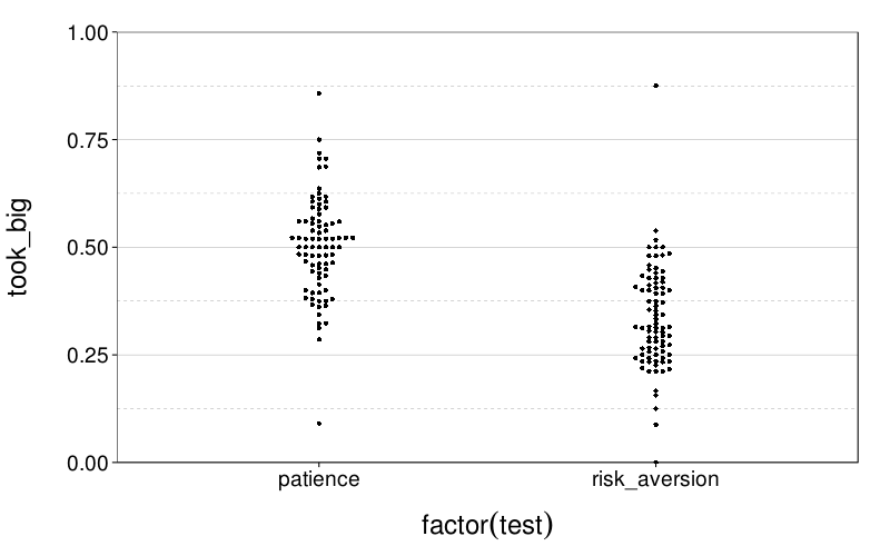
Choice proportions for all sessions, collapsing across subjects:
dodge(factor(test), took_big, data =
        aggregate(took_big ~ sesn + s + test, econg, mean)) +
    coord_cartesian(ylim = c(0, 1))
Let's score the econometric tests simply by picking indifference values through logistic regression. Indifference values are expressed as ratios; specifically, as the small amount divded by the big amount.
eips = econ.indiff.per.sess(econg)
First, collapsing across all sessions:
dodge(factor(test), y, data = ss(eips, test != "stationarity")) +
    boxp
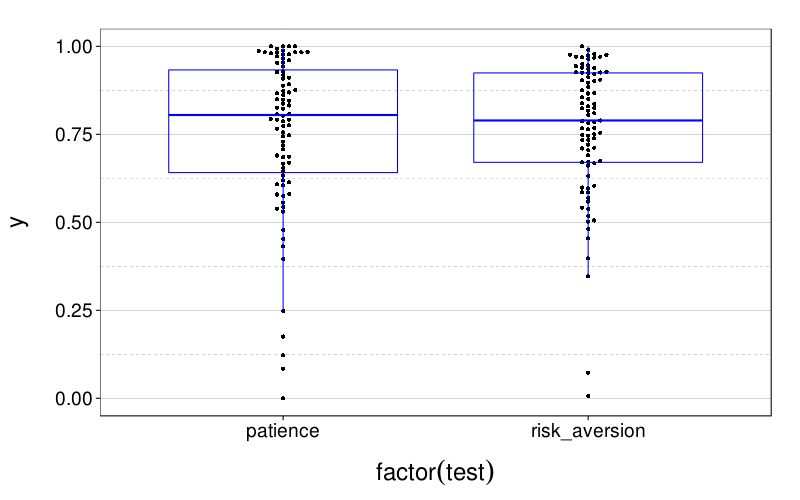
It looks like .75 would be a better initial guess for the discount factors in both tests.
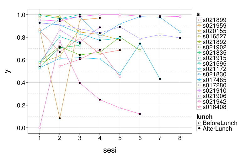
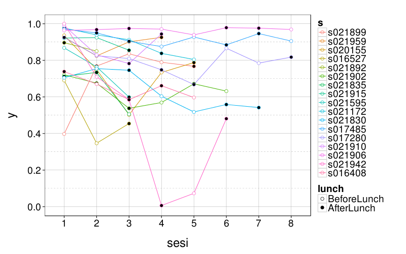
Now, session-by-session:
econ.sess.plot(ss(eips, test == "patience"))
econ.sess.plot(ss(eips, test == "risk_aversion"))
Test–retest reliability
First, here are some reliability figures for time-preference tests obtained in different studies. All the tests are different, of course.
- Matusiewicz, Carter, Landes, and Yi (2013): r = .70 for hypothetical rewards, 1-week interval
- Kirby (2009): Using a pretty coarse response scale, r = .77 for 1 week and r = .71 for 1 year
- Beck and Triplett (2009): r = .64 for and r = .70 for AUC, 6-week interval
- Ohmura, Takahashi, Kitamura, and Wehr (2006): r = .60 for hyperbolic and r = .75 for AUC, 3-month interval
Here, for the sake of simplicity, we'll treat the same subject in the two hunger conditions as two different subjects.
retest.eips = function(eips)
   {eips = ss(eips,
        table(paste(s, hungry))[paste(s, hungry)] > 1)
    levs = with(
         ordf(
            ddply(eips, .(s, hungry), function(slice)
                cbind(slice, my = median(slice$y))),
            my),
         unique(paste(s, hungry)))
    list(
        medrange = median(with(eips, tapply(y, paste(s, hungry),
            function(y) max(y) - min(y)))),
        plot = qplot(match(paste(s, hungry), levs), y, data = eips) +
            stat_summary(fun.ymin = min, fun.ymax = max,
                color = "red", geom = "linerange") +
            scale_y_continuous(breaks = seq(0, 1, .2)) +
            scale_x_continuous(breaks = c()))}
retest.eips(ss(eips, test == "patience"))$plot
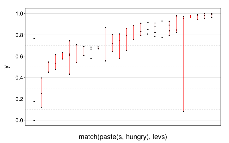
Here's the median of these ranges:
round(d = 3, retest.eips(ss(eips, test == "patience"))$medrange)
| value | |
|---|---|
| 0.133 |
Doesn't seem too bad.
To get a number comparable to the usual correlation coefficients used to express reliability, let's estimate the variance components and see what correlation they imply.
varcov = VarCorr(type = "varcov", lmer(
    y ~ 1 + (1 | g),
    data = transform(ss(eips, test == "patience"),
        g = droplevels(interaction(s, hungry)))))
errvar = attr(varcov, "sc")^2
gvar = as.numeric(varcov)
round(d = 3, gvar / (gvar + errvar))
| value | |
|---|---|
| 0.561 |
That's pretty low.
retest.eips(ss(eips, test == "risk_aversion"))
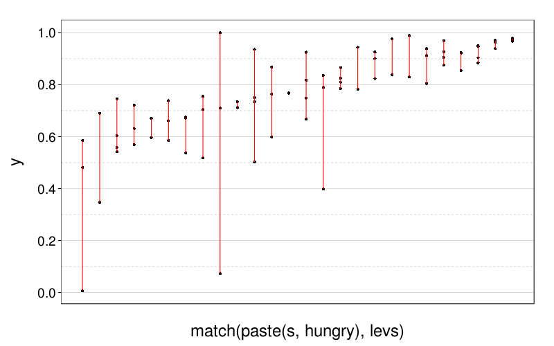
round(d = 3, retest.eips(ss(eips, test == "risk_aversion"))$medrange)
| value | |
|---|---|
| 0.145 |
But that plot I don't like as much.
varcov = VarCorr(type = "varcov", lmer(
    y ~ 1 + (1 | g),
    data = transform(ss(eips, test == "risk_aversion"),
        g = droplevels(interaction(s, hungry)))))
errvar = attr(varcov, "sc")^2
gvar = as.numeric(varcov)
round(d = 3, gvar / (gvar + errvar))
| value | |
|---|---|
| 0.434 |
Even lower than for patience.
Differences between conditions
Greater patience scores mean greater patience, so if hunger decreases patience (as we expect), before < after and hence before - after < 0.
dodge(1, before - after, data = ddply(
    ss(eips, test == "patience" & !is.na(lunch)), .(s),
    function(slice) data.frame(
        before = mean(ss(slice, lunch == "BeforeLunch")$y),
        after = mean(ss(slice, lunch == "AfterLunch")$y)))) +
    ylab("Effect of hunger on patience")
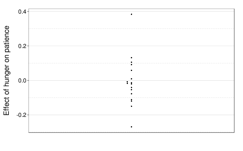
At least this difference is in the right direction.
For risk aversion, greater risk_aversion scores actually mean less risk aversion (i.e., more risk-taking), since the score is supposed to give the discount factor for a gain with 95% probability compared to a certain gain. Thus if hunger increases risk-taking (as we expect), before > after for risk_aversion, and hence before - after > 0.
dodge(1, before - after, data = ddply(
    ss(eips, test == "risk_aversion" & !is.na(lunch)), .(s),
    function(slice) data.frame(
        before = mean(ss(slice, lunch == "BeforeLunch")$y),
        after = mean(ss(slice, lunch == "AfterLunch")$y)))) +
    ylab("Effect of hunger on risk-taking")
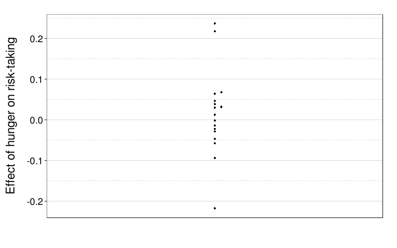
Looks about evenly split.
References
Beck, R. C., & Triplett, M. F. (2009). Test–retest reliability of a group-administered paper–pencil measure of delay discounting. Experimental and Clinical Psychopharmacology, 17, 345–355. doi:10.1037/a0017078
Kirby, K. N. (2009). One-year temporal stability of delay-discount rates. Psychonomic Bulletin and Review, 16(3), 457–462. doi:10.3758/PBR.16.3.457
Matusiewicz, A. K., Carter, A. E., Landes, R. D., & Yi, R. (2013). Statistical equivalence and test–retest reliability of delay and probability discounting using real and hypothetical rewards. Behavioural Processes, 100, 116–122. doi:10.1016/j.beproc.2013.07.019
Ohmura, Y., Takahashi, T., Kitamura, N., & Wehr, P. (2006). Three-month stability of delay and probability discounting measures. Experimental and Clinical Psychopharmacology, 14(3), 318–328. doi:10.1037/1064-1297.14.3.318